

Can a machine-learning model appear reliable because its preprocessing has already seen the test set? This failure is called data leakage. It occurs when information that should remain unavailable during training influences feature engineering, model selection, or evaluation. The resulting score may look impressive while overstating how the system will behave on genuinely unseen data.
Scikit-learn pipelines address an important part of this problem structurally. They connect preprocessing and estimation in one object, ensuring that each transformation is fitted at the correct point in training and cross-validation. In this article, you will examine the distinction between fit and transform, reproduce a numerical leakage example, and build a complete pipeline for mixed numerical and categorical data.
Open the executed notebook in Google Colab
Why must you split data before preprocessing?
A test set is a proxy for future observations. Its purpose is to estimate how a trained system will perform on data that played no role in model development. Once a statistic from that set influences training, the boundary between training and evaluation has been weakened.
Consider standardization. To transform a value $x$ into a standardized value $z$, StandardScaler uses a mean $\mu$ and a standard deviation $\sigma$:
\[ z = \frac{x – \mu}{\sigma} \]
If $\mu$ and $\sigma$ are calculated from the complete dataset, the test observations influence the coordinate system in which the model is trained. Their labels may never be exposed, but information about their feature distribution has already entered the process. This is why leakage can occur without an obvious programming error or direct access to the target.
The safe order is therefore:
- define the features and target;
- create the train-test split;
- fit every learned transformation on the training set;
- apply those fitted transformations to the test set;
- evaluate the model once on the untouched test data.
The companion notebook uses the Titanic dataset distributed through Seaborn. It retains survival as the target and five predictors: passenger class, sex, age, fare, and port of embarkation.
import seaborn as sns
from sklearn.model_selection import train_test_split

df = sns.load_dataset("titanic")
columns = ["survived", "pclass", "sex", "age", "fare", "embarked"]
df = df[columns]

X = df.drop(columns="survived")
y = df["survived"]

X_train, X_test, y_train, y_test = train_test_split(
    X, y, test_size=0.2, stratify=y, random_state=42
)
With this deterministic split, the executed notebook contains 712 training passengers and 179 test passengers. The original data also contain 177 missing ages and two missing embarkation values. Those missing values are useful here because imputation is itself a learned transformation and can leak information when applied in the wrong order.
What do fit, transform, and fit_transform actually do?
Scikit-learn transformers follow a consistent interface. fit learns state from data: a mean, a median, a vocabulary of categories, principal components, selected features, or another set of parameters. transform applies the operation using the state that has already been learned. fit_transform performs both steps on the same input and is typically used on training data.
The distinction is more than API vocabulary. It encodes which information an object is allowed to learn. In the manual standardization example, each scaler is fitted only on non-missing training values:
from sklearn.preprocessing import StandardScaler

age_scaler = StandardScaler().fit(X_train[["age"]].dropna())
fare_scaler = StandardScaler().fit(X_train[["fare"]].dropna())

print(age_scaler.mean_[0], age_scaler.scale_[0])
print(fare_scaler.mean_[0], fare_scaler.scale_[0])
The executed result gives an age mean of 29.81 with a standard deviation of 14.47, and a fare mean of 31.82 with a standard deviation of 48.03. These values become fitted attributes of the scaler. When the test set is transformed later, the training mean and standard deviation are reused; the test set does not receive a new coordinate system.
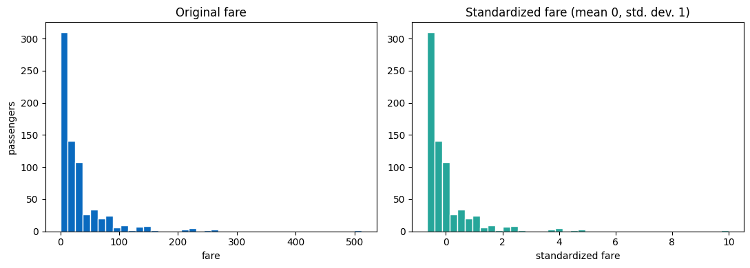
Standardization changes location and scale, not the underlying shape of the fare distribution. The plot was generated by the executed English notebook.
The long right tail remains visible after standardization. This matters because scaling is not a general remedy for skewness or outliers. It places features on comparable numerical scales, which can improve the optimization of models such as logistic regression and support vector machines, but it does not make a distribution Gaussian.
How can a small numerical difference invalidate an evaluation?
Leakage is often difficult to notice because the contaminated value may remain plausible. The notebook fits one fare scaler correctly on X_train and another incorrectly on all observations:
correct_scaler = StandardScaler().fit(X_train[["fare"]].dropna())
leaked_scaler = StandardScaler().fit(X[["fare"]].dropna())

print(correct_scaler.mean_[0])
print(leaked_scaler.mean_[0])
The training-only mean is 31.8198; the leaked mean is 32.2042. A difference of less than one monetary unit may seem harmless, but magnitude is not the governing principle. The second calculation uses information from the 179 held-out passengers before evaluation begins.
The effect becomes more consequential when preprocessing is sensitive to the empirical distribution. Examples include target encoding, feature selection, outlier thresholds, high-dimensional dimensionality reduction, nearest-neighbor imputation, and resampling. In these settings, a seemingly modest leak can change the representation or even which features enter the model.
The scikit-learn guide to common pitfalls makes the same point: preprocessing decisions must be learned from the appropriate training subset and then applied consistently to later data.
How does ColumnTransformer handle mixed feature types?
Real tables rarely contain one homogeneous feature type. Age and fare are numerical, while passenger class, sex, and embarkation port are categorical. Each group requires a different sequence of operations.
For the numerical branch, the notebook fills missing values with the training median and then standardizes the result. For the categorical branch, it fills missing values with the most frequent training category and applies one-hot encoding. handle_unknown="ignore" prevents an unseen category at inference time from causing an exception.
from sklearn.compose import ColumnTransformer
from sklearn.impute import SimpleImputer
from sklearn.pipeline import Pipeline
from sklearn.preprocessing import OneHotEncoder, StandardScaler

numeric_features = ["age", "fare"]
categorical_features = ["pclass", "sex", "embarked"]

numeric_transformer = Pipeline(steps=[
    ("imputer", SimpleImputer(strategy="median")),
    ("scaler", StandardScaler()),
])

categorical_transformer = Pipeline(steps=[
    ("imputer", SimpleImputer(strategy="most_frequent")),
    ("encoder", OneHotEncoder(handle_unknown="ignore")),
])

preprocessor = ColumnTransformer(transformers=[
    ("numeric", numeric_transformer, numeric_features),
    ("categorical", categorical_transformer, categorical_features),
])
The important property is not only convenience. Both imputers and the scaler remain inside an estimable object. When preprocessor.fit(X_train) is called, every learned quantity comes from the training data. The fitted object can then apply the same transformations to validation, test, or production observations.
This composition also preserves columns that require different representations without forcing them into separate manual workflows. The official documentation on pipelines and composite estimators describes this design as a way to assemble several transformations and a final estimator while exposing a unified interface.
How does a scikit-learn pipeline prevent leakage?
The final estimator connects preprocessor to logistic regression:
from sklearn.linear_model import LogisticRegression

model = Pipeline(steps=[
    ("preprocessing", preprocessor),
    ("classifier", LogisticRegression(max_iter=1000)),
])

model.fit(X_train, y_train)

print(model.score(X_train, y_train))
print(model.score(X_test, y_test))
One call to fit now learns the imputation values, scaling parameters, encoded categories, and classifier coefficients in the correct order. The executed notebook reports 0.801 training accuracy and 0.771 test accuracy.
Those two numbers are close, but this alone does not prove that the model generalizes or that logistic regression is optimal for the problem. It only shows that the demonstration does not exhibit a large training-test accuracy gap. The stronger claim is procedural: because the test set did not participate in fitting any step, the reported test accuracy is a legitimate held-out estimate for this specific split.
The pipeline also defines an operational contract. model.predict(new_data) first applies the fitted preprocessing and then computes the prediction. There is no need to reproduce scaling, imputation, and encoding in a separate production script. The same fitted object can be serialized, versioned, and tested as one unit.
Why are pipelines essential during cross-validation?
Cross-validation does not remove leakage automatically. Suppose you standardize the complete training set and only then call cross_val_score. Each validation fold has already influenced the scaling parameters used by the other folds. The outer test set remains untouched, but the cross-validation estimate used for model selection is contaminated.
When the entire pipeline is passed to cross_val_score, scikit-learn clones and fits it inside each training fold. The preprocessing state is therefore relearned five times in a five-fold evaluation:
from sklearn.model_selection import cross_val_score

scores = cross_val_score(
    model, X_train, y_train, cv=5, scoring="accuracy"
)
The executed scores are 0.790, 0.762, 0.796, 0.831, and 0.810, for a mean accuracy of 0.798 ± 0.023. Their proximity to the held-out test accuracy is reassuring, although it should not be overinterpreted: five folds on one modest dataset do not characterize every subgroup, threshold, or deployment condition.
If hyperparameters are tuned, the same principle extends to model selection. Keep preprocessing inside the estimator supplied to GridSearchCV or RandomizedSearchCV. For an unbiased final estimate after extensive tuning, retain a separate test set or use nested cross-validation. The scikit-learn cross-validation guide details these evaluation patterns.
What does a pipeline not protect you from?
A pipeline prevents leakage only for operations placed inside it and evaluated with a correct splitting strategy. It cannot repair information that was already introduced upstream.
Several risks remain:
- Temporal leakage: a random split may allow future observations to inform a model intended to predict the past. Time-dependent problems need chronological validation.
- Group leakage: records from the same patient, customer, device, or site may appear in both training and validation sets. Group-aware splitting is required.
- Target-derived features: a feature calculated from the label, or from data collected after the prediction moment, remains invalid even when wrapped in a pipeline.
- Duplicate entities: near-duplicate images, documents, or transactions can make train and test sets artificially similar.
- Selection on the test set: repeatedly checking the test score and changing the model turns the test set into an informal validation set.
The pipeline is therefore a mechanism for enforcing transformation boundaries, not a substitute for understanding how data were generated. A reliable evaluation begins by defining the unit of independence, the prediction moment, and the operational population before choosing a splitter.
Takeaways
- Split before fitting transformations. The test set must not influence means, medians, categories, selected features, or any other learned preprocessing state.
fitlearns;transformapplies. This distinction determines which data contribute information to a transformer.- A small leaked statistic still invalidates the boundary. The issue is unauthorized information flow, not only the numerical size of the difference.
ColumnTransformergives each feature type its own path. Numerical and categorical preprocessing remain explicit while sharing one fitted interface.Pipelinejoins preprocessing and estimation. The same object can support training, validation, prediction, persistence, and deployment.- Cross-validation must refit preprocessing inside every fold. Passing the complete pipeline to model-selection tools preserves this isolation.
- Data design remains decisive. Temporal, grouped, duplicated, or target-derived information requires a splitting strategy that reflects the real prediction task.