

How can a collection of ordinary photographs become a set of cameras positioned in space and, eventually, a three-dimensional point cloud? Before a reconstruction system can estimate depth, it must solve a more fundamental problem: identify evidence that the same physical point appears in different images. This is where feature detection for 3D reconstruction begins.
A feature detector finds repeatable local structures—corners, textured details, and distinctive regions—and represents them numerically. Multiview geometry can then test those candidate correspondences, reject inconsistent matches, and triangulate points. Without reliable 2D evidence, a Structure from Motion (SfM) pipeline has no geometric foundation.
This article examines SIFT, explains how COLMAP organizes feature extraction and matching, and interprets measured results from the South Building dataset. The companion notebook uses OpenCV to make the detector observable while preserving a clear boundary between an instructional experiment and a complete SfM implementation.
Open the executed notebook in Google Colab
What is feature detection for 3D reconstruction?
A camera projects a three-dimensional scene onto a two-dimensional sensor. For a homogeneous image coordinate  , measured in pixels, and a homogeneous 3D point
  , the camera model can be written as
![\[ \mathbf{u} \sim \mathbf{K}[\mathbf{R}\mid\mathbf{t}]\mathbf{X}, \]](https://sigmoidal.ai/wp-content/ql-cache/quicklatex.com-da1e3a5dd1679b0172adc953fcb684b0_l3.png "Rendered by QuickLaTeX.com")
where  contains the intrinsic camera parameters, while
  and
and  describe the camera pose. A single image identifies the direction of a projection ray, but it does not determine the distance to the observed point. Depth emerges only when compatible observations from multiple viewpoints are combined. If you want to examine this model in greater detail, the English guide to matrix transformations and camera coordinate systems develops the underlying geometry.
Reconstruction therefore depends on a sequence of inferences rather than one operation:
- Detect repeatable features in each photograph.
- Describe and match those features across image pairs.
- Verify the geometry of the matches and remove accidental associations.
- Estimate camera poses, triangulate points, and optimize the model through bundle adjustment.
The COLMAP command-line interface exposes this structure directly through its feature_extractor, matching tools, and mapper. The geometry at the end of the pipeline depends both on how the photographs were captured and on the reliability of the initial correspondences.
What separates a keypoint from a descriptor?
A keypoint is a location accompanied by local geometric attributes such as image position, scale, and, for many detectors, orientation. A descriptor is the numerical representation of the neighborhood around that location. Their roles are distinct but complementary: the keypoint determines where to inspect, while the descriptor supports comparisons across images.
A smooth wall or a clear area of sky provides little local evidence because many pixels have similar neighborhoods. A window corner, brick junction, or architectural ornament produces intensity changes in more than one direction. These structures are more likely to remain identifiable under moderate changes in viewpoint, scale, and illumination.
This distinction also prevents a common misunderstanding. A large number of keypoints does not guarantee a successful reconstruction. Features must be repeatable, their descriptors must remain compatible between views, and the resulting matches must satisfy the geometry of the camera pair. The detector supplies candidates; it does not create 3D points by itself.
Why does SIFT remain relevant?
The Scale-Invariant Feature Transform (SIFT), introduced by David Lowe, detects local structures across multiple scales and assigns a dominant orientation to each retained point. Its traditional descriptor contains 128 components built from histograms of gradient orientations around the keypoint. The complete method is described in the original SIFT paper.
The procedure begins with scale space. For an image  , Gaussian filters are applied at different values of
  :
:
![\[ L(x,y,\sigma)=G(x,y,\sigma)\ast I(x,y). \]](https://sigmoidal.ai/wp-content/ql-cache/quicklatex.com-a55f722a3cfe39246101356178c15085_l3.png "Rendered by QuickLaTeX.com")
The Difference of Gaussians (DoG) then provides an efficient approximation to the scale-normalized Laplacian of Gaussian response:
![\[ D(x,y,\sigma)=L(x,y,k\sigma)-L(x,y,\sigma). \]](https://sigmoidal.ai/wp-content/ql-cache/quicklatex.com-4d00c670bbb058d3efe1a3c5cda6572a_l3.png "Rendered by QuickLaTeX.com")
Local extrema in the position–scale volume become keypoint candidates. A complete SIFT implementation refines their locations, rejects unstable edge responses, assigns one or more orientations, and constructs normalized descriptors with interpolation. This sequence explains why SIFT is more robust than direct pixel comparison when the camera rotates, the image scale changes, or illumination varies moderately.
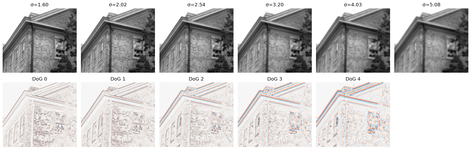
Scale space and Difference of Gaussians for the crop used in the notebook. The figure illustrates the principle; OpenCV’s tested SIFT implementation performs the feature extraction.
What does the executed notebook establish?
The notebook applies cv2.SIFT_create() to an architectural crop from the South Building dataset. In the recorded execution with Python 3.12.3 and OpenCV 4.11.0, the detector found 10,982 keypoints and returned a descriptor matrix with shape (10,982, 128) in float32 format.
The core operation is deliberately concise:
sift = cv2.SIFT_create()
keypoints, descriptors = sift.detectAndCompute(image_gray, None)
detectAndCompute performs two related tasks. It first locates keypoints and estimates their scale and orientation; it then computes the 128-dimensional descriptor for each retained location. The circles in the visualization encode location and scale, while the radial marks indicate orientation.
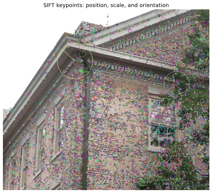
Keypoints concentrate around bricks, windows, roof lines, and foliage—regions that provide distinctive local intensity patterns.
The count belongs to this crop, parameterization, and OpenCV version. It is not an intrinsic property of the dataset. In a separate COLMAP execution over the 128 South Building photographs, the observed mean was 11,148 features per image, with a median of 11,508. Image resolution, extraction settings, and scene content all influence those values.
Spatial distribution matters as well. Two bands with the same area produced very different counts: the upper third contained 2,023 keypoints, while the lower third contained 4,579, a ratio of 2.26. This comparison does not measure match quality. It shows where the crop offers more candidate evidence.
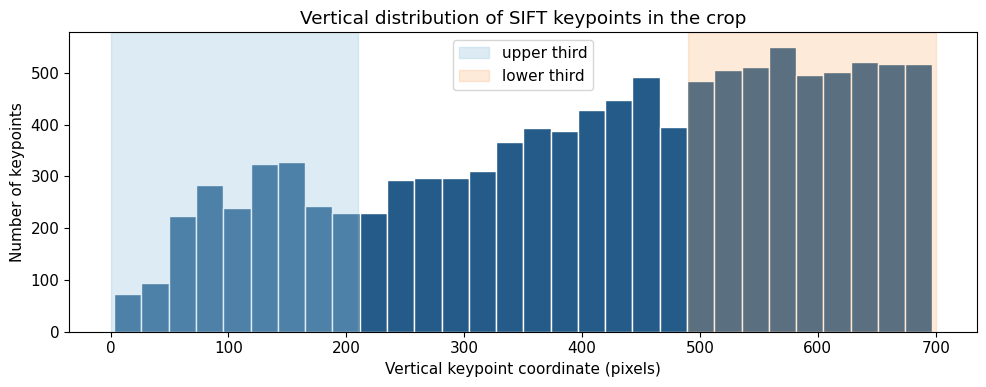
The lower third contains more detected keypoints than the upper third because the visible architecture and vegetation provide denser local texture.
How do descriptors become reliable correspondences?
After extraction, the system compares descriptors between images. A small distance between two 128-dimensional vectors is only a hypothesis that both observations correspond to the same physical point. Repeated windows, reflections, moving objects, and similar textures can produce convincing but incorrect matches.
Geometric verification is therefore indispensable. For two calibrated views, let  denote normalized homogeneous image coordinates. Valid correspondences satisfy the epipolar constraint defined by the essential matrix
  :
:
![\[ \mathbf{x}_2^\top\mathbf{E}\mathbf{x}_1=0. \]](https://sigmoidal.ai/wp-content/ql-cache/quicklatex.com-18f2696062469ff377d498dbaeb57653_l3.png "Rendered by QuickLaTeX.com")
In pixel coordinates, the equivalent relationship uses the fundamental matrix  . Robust estimators such as RANSAC fit the model while rejecting outliers. Only the surviving inliers should contribute to pose recovery and triangulation.
The complete COLMAP experiment processed all 8,128 possible image pairs from the 128-image collection. Of those pairs, 2,610 produced a verified two-view geometry; the smallest accepted set contained 15 inliers. Processing a pair and obtaining a useful geometric relationship are not equivalent outcomes.
The mean connectivity was 40.8 images per photograph, and no image remained isolated. With that connected evidence, the mapper registered 128 of 128 images in one sparse model, triangulated 84,956 3D points, and reported a mean reprojection error of 0.61 pixel. These figures describe one dataset and configuration. They should not be converted into universal thresholds for calibration or reconstruction quality.
This incremental mapping strategy follows the system described by Schönberger and Frahm in Structure-from-Motion Revisited. For a broader historical example of scaling the same class of problem, see the English article on reconstructing Rome from large photo collections.
Where does the classical pipeline tend to fail?
The behavior of the detector exposes the limitations of classical SfM. Sky, textureless walls, and transparent surfaces offer little stable local evidence. Foliage may move between photographs. Windows and metal surfaces introduce reflections that violate the assumption of consistent appearance. Repetitive patterns make descriptor matches ambiguous even when each individual patch is visually distinctive.
Capture strategy is therefore part of the algorithmic system. Sufficient overlap, controlled motion blur, viewpoint diversity, and exposure consistency improve the probability that features remain both detectable and matchable. A detector cannot recover evidence that the photographs never recorded.
Recent methods such as NeRF and Gaussian Splatting model scene appearance differently, but they do not make camera geometry irrelevant. Conventional pipelines often receive poses estimated by SfM or incorporate an equivalent pose-optimization procedure. Reliable correspondences remain one of the most established ways to construct that geometric foundation.
What does this notebook implement—and what does it omit?
The public notebook is intentionally explicit about its scope. It uses OpenCV’s SIFT implementation to produce keypoints and descriptors. The scale-space and DoG cells explain the mathematical intuition, but they do not reproduce Lowe’s full algorithm or COLMAP’s complete feature-extraction and mapping pipeline.
That separation makes the experiment more useful. You can inspect the structures that motivate the detector while relying on a tested implementation for the measured outputs. For production SfM work, use established libraries, validate the complete pipeline, and examine the distribution of errors and scene coverage rather than promoting an instructional implementation into an operational dependency.
Takeaways
- Feature detection is the entry point to 3D reconstruction. It provides local observations that can be matched across images; without reliable correspondences, triangulation is not robust.
- Keypoints and descriptors serve different purposes. A keypoint locates a structure, while a descriptor supports comparison with observations from another view.
- SIFT seeks stability across scale and orientation. Scale space, DoG, localization, orientation assignment, and gradient histograms work together.
- Counts require context. Feature totals and reprojection errors describe a particular experiment, not universal quality thresholds.
- The detector is only the beginning. Matching, geometric verification, pose estimation, triangulation, and bundle adjustment are all necessary to convert 2D evidence into 3D structure.