Detecting Image Blur with FFT in Python

Can a computer-vision pipeline reject a blurred frame before that frame reaches a detector, classifier, or measurement system? One practical answer is to examine what blur removes: the fine spatial variations associated with edges and texture.

A sharp image contains intensity transitions at several spatial scales. Blur suppresses the faster transitions, so its effect becomes especially visible in the frequency domain. The Fast Fourier Transform (FFT) provides a direct way to isolate those high-frequency components and turn them into a measurable sharpness score.

This article develops a global FFT blur detector in Python, validates it under progressively stronger Gaussian blur, and compares its response with the variance of the Laplacian. The accompanying experiment is deliberately controlled: it explains the mechanism and its failure modes rather than presenting one threshold as a universal production rule.

Open the executed notebook in Google Colab

Why can the Fourier transform detect image blur?

Suppose that an observed image is produced by convolving a sharp image with a point-spread function :

   

The convolution theorem turns this spatial operation into multiplication in the frequency domain:

   

For Gaussian blur, behaves as a low-pass filter. Components near the zero-frequency center are preserved more strongly, while components farther from the center are attenuated. Those outer components encode rapid changes in image intensity: edges, small structures, and fine texture.

The visual difference is clear when the same subject is photographed under two focus conditions.

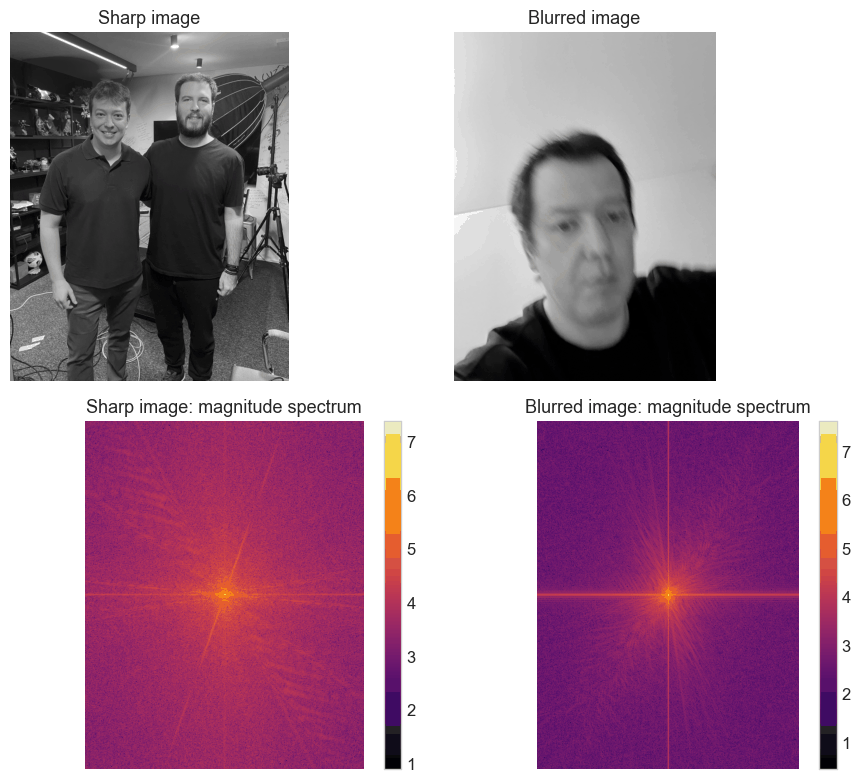
The blurred photograph concentrates more of the visible magnitude near the low-frequency center. The displayed values use a logarithmic scale so weak and strong components can be inspected together.

This observation needs one technical qualification. The detector below does not compute spectral energy in the strict signal-processing sense, which would normally involve squared magnitude. It computes the mean absolute amplitude of a spatial signal reconstructed after low frequencies have been removed. That quantity is a useful focus score, but its units and threshold depend on the image preparation and the scene.

The approach is related to a broader literature on spectral blur features. For example, Liu, Li, and Jia developed a patch-based framework for partial-blur detection and classification in Image Partial Blur Detection and Classification. Our global score is an instructional baseline inspired by frequency analysis; it is not a reproduction of their learned patch classifier.

How does the FFT blur detector work?

The detector converts a grayscale image into a scalar score through five operations:

1. Compute the two-dimensional FFT with np.fft.fft2.
2. Center the zero-frequency component with np.fft.fftshift.
3. Set a circular region around that center to zero, removing low spatial frequencies.
4. Apply the inverse FFT to reconstruct the retained high-frequency signal.
5. Average its absolute amplitude and compare the result with a calibrated threshold.

A circular mask is appropriate because distance from the centered origin represents spatial-frequency magnitude independently of orientation. A square exclusion region would treat diagonal and axial frequencies differently at the same radial distance.

The implementation is compact:

def detect_blur_fft(image, size=60, threshold=5):
    """Measure retained high-frequency magnitude in a grayscale image."""
    if image.ndim != 2:
        raise ValueError("The input must be a two-dimensional grayscale image.")

    height, width = image.shape
    center_y, center_x = height // 2, width // 2

    shifted = np.fft.fftshift(np.fft.fft2(image))

    y_coordinates, x_coordinates = np.ogrid[:height, :width]
    radius = np.sqrt(
        (x_coordinates - center_x) ** 2
        + (y_coordinates - center_y) ** 2
    )
    shifted[radius <= size] = 0

    reconstructed = np.fft.ifft2(np.fft.ifftshift(shifted))
    mean_magnitude = float(np.mean(np.abs(reconstructed)))
    return mean_magnitude, mean_magnitude <= threshold

The executed notebook resizes both references to 500 pixels in width, uses a mask radius of 60 frequency bins, and sets the decision threshold to 5. It also verifies the SHA-256 hashes of the downloaded photographs before decoding them. Under those exact conditions, the sharp image produces a score of 9.03, while the blurred image produces 2.30. Both classifications match the expected labels.

These values establish that the chosen configuration separates this pair. They do not establish that 5 is a suitable threshold for another camera, resolution, scene family, or preprocessing pipeline.

What happens as Gaussian blur increases?

A two-image comparison could succeed by chance because image content and focus differ simultaneously. A more informative experiment starts with one fixed image and applies Gaussian kernels of increasing size. This preserves the scene while changing the amount of smoothing.

The notebook evaluates odd kernel sizes from 1 through 31. The FFT score begins at 9.03 for the unchanged image, falls to 6.00 at kernel 3, crosses the selected threshold at 4.81 for kernel 5, and reaches 0.89 at kernel 31.

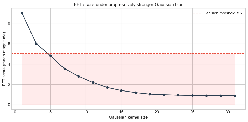
The score decreases monotonically in this controlled sequence. The shaded region indicates the values classified as blurred by the illustrative threshold.

The English notebook contains an assertion that verifies this monotonic decrease. That test is useful because it protects a specific empirical claim in the article: if a future dependency or code change alters the output, execution stops instead of silently publishing inconsistent numbers.

The curve also reveals why threshold calibration matters. A threshold of 5 declares kernel 5 blurred and kernel 3 sharp. That boundary may be reasonable for these images, but an industrial inspection system might reject subtler loss of focus, while a video analytics system might tolerate more smoothing to avoid discarding too many frames.

The mask radius has a similar interpretation. Increasing size removes a wider central band and measures only more extreme high frequencies. Decreasing it retains lower-frequency structures. Because size=60 is expressed in discrete frequency bins, resizing the image without reconsidering this value changes what the detector measures.

How does FFT compare with the variance of the Laplacian?

The variance of the Laplacian is a widely used spatial-domain focus measure. The Laplacian approximates a second derivative, producing strong responses around rapid intensity changes. A sharp, textured image therefore tends to have higher response variance than a smoothed version.

With OpenCV, the metric requires one line:

def laplacian_variance(image):
    return float(cv2.Laplacian(image, cv2.CV_64F).var())

Laplacian-based focus measures have been evaluated in autofocus research, including the comparison by Pech-Pacheco and colleagues in Diatom Autofocusing in Brightfield Microscopy. The method is attractive because it uses a local convolution and avoids an FFT mask parameter.

The two metrics have different scales, so the notebook divides each sequence by its value at kernel 1. The resulting curves compare relative response, not absolute scores.

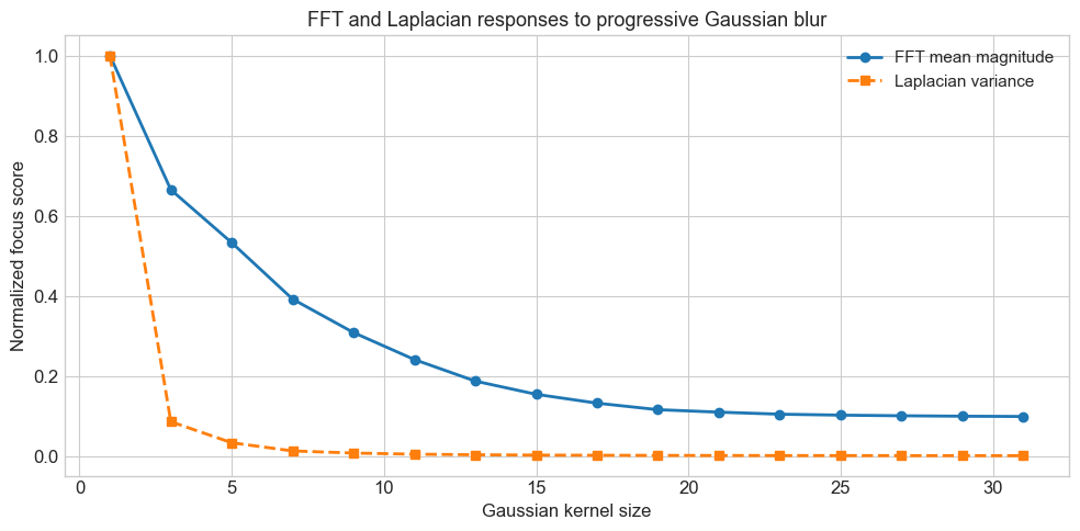
At kernel 5, the normalized FFT score is 0.533, while normalized Laplacian variance is 0.033. This result describes one image and one Gaussian sequence, not a general accuracy benchmark.

The Laplacian reacts much more sharply to the first smoothing steps in this experiment. The FFT score decays more gradually, preserving separation among stronger blur levels. Neither response is intrinsically superior. A binary quality gate may benefit from the Laplacian’s sensitivity, while a graded focus indicator may benefit from a smoother response. The decision should follow validation against the errors that matter in the target application.

Computational cost can also matter. A local Laplacian filter scales linearly with the number of pixels for a fixed kernel, while a two-dimensional FFT scales approximately as for an image. Actual latency still depends on implementation, image size, hardware, and whether the Fourier representation is already needed elsewhere in the pipeline.

Where can a global blur score fail?

Frequency content is influenced by more than focus. Several failure modes deserve explicit tests:

• Low-texture scenes: a clear sky, blank wall, or defocused background may contain little high-frequency content even when captured correctly, producing a false positive.
• Partial blur: a global average can hide a blurred region surrounded by sharp content. Patch-level evaluation is more suitable when local focus matters.
• Motion blur: directional motion produces an anisotropic spectral signature, unlike the isotropic Gaussian smoothing used in the controlled experiment.
• Noise: sensor noise contributes high-frequency components and can make a blurred image appear sharper to either metric.
• JPEG compression: block boundaries introduce artificial high frequencies that can inflate a score.
• Image boundaries: the discrete Fourier transform treats the image as periodic. Discontinuities between opposite borders can create spectral leakage; windowing may reduce this effect, although it also changes the score.
• Resolution changes: resizing, cropping, and sharpening alter the frequency distribution and therefore require recalibration.

A production threshold should be selected from a labeled dataset collected with the intended camera and preprocessing path. Normalize image dimensions, calculate the score for sharp and unacceptable examples, inspect precision-recall or ROC curves, and choose the operating point according to the cost of false rejection versus missed blur. Then reserve a separate validation set for the final estimate.

When one scalar is insufficient, combine complementary evidence. Patch-level FFT or Laplacian scores can localize defects; edge-density or gradient measures can account for scene texture; metadata such as exposure time can identify motion risk; and a learned model can represent blur types that handcrafted metrics do not separate well.

Takeaways

• Blur suppresses high spatial frequencies: Gaussian smoothing concentrates more of the visible Fourier magnitude near the low-frequency center.
• The FFT detector is a high-pass focus score: it removes a circular low-frequency region, reconstructs the retained signal, and measures its mean absolute amplitude.
• The controlled outputs are reproducible: the sharp and blurred references score 9.03 and 2.30, and the progressive sequence decreases monotonically from 9.03 to 0.89.
• Laplacian variance responds more abruptly in this experiment: at kernel 5, its normalized value is 0.033 versus 0.533 for the FFT score.
• No threshold is universal: resolution, scene texture, noise, compression, and acquisition conditions all affect the result.
• Classical metrics remain valuable baselines: they are interpretable, inexpensive to validate, and useful as quality-control gates when their limitations are measured explicitly.