


Why should a confidently wrong prediction receive a much larger penalty than an uncertain one? Binary cross-entropy answers this question by evaluating probabilities, not merely final class labels. A model that assigns 99% probability to the wrong class has made a fundamentally different error from a model that remains near 50%.
This distinction connects probability theory, optimization, and classification. Starting with a Bernoulli model for binary outcomes, we can derive binary cross-entropy as a negative log-likelihood, obtain the gradient used to train logistic regression, and interpret the resulting decision boundary. The mathematics, implementation, outputs, and limitations form one complete technical argument.
Open the executed notebook in Google Colab
Why is a linear score not a probability?
Suppose a model must predict whether an observation belongs to class 0 or class 1. The target is binary, $y \in \{0,1\}$, but a linear model produces an unrestricted score:
\[z = w^\top x + b\]
The score $z$ can assume any real value. That makes it unsuitable as a probability, which must lie between zero and one. Applying an arbitrary threshold to the raw score would produce class labels, but it would not provide a coherent probabilistic model.
Logistic regression solves this problem with the sigmoid function:
\[\sigma(z) = \frac{1}{1 + e^{-z}}\]
The sigmoid maps the entire real line to the open interval $(0,1)$. Its output can therefore be interpreted as the conditional probability of the positive class:
\[\hat{p} = P(y=1 \mid x; w,b) = \sigma(w^\top x+b)\]
When $z=0$, the model produces $\hat{p}=0.5$. Positive scores move the probability toward one, while negative scores move it toward zero. The value before the sigmoid is often called a logit. In fact, the log-odds are linear in the features:
\[\log\left(\frac{\hat{p}}{1-\hat{p}}\right)=w^\top x+b\]
The companion notebook creates 200 observations from two partially overlapping Gaussian clusters. The overlap matters: it prevents the example from becoming a trivial geometric separation problem and gives the probability surface a meaningful transition region.
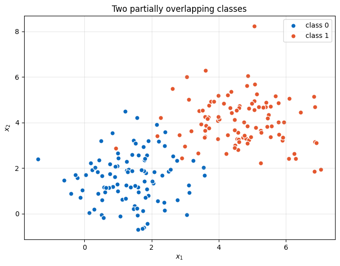
The experiment contains 100 observations from each class. The two features are synthetic and have no physical units.
How does Bernoulli likelihood become binary cross-entropy?
A single binary outcome can be represented with a Bernoulli distribution. Given the predicted probability $\hat{p}$, the probability of observing $y$ is
\[p(y \mid x;w,b)=\hat{p}^{\,y}(1-\hat{p})^{1-y}\]
The exponents select the appropriate term. If $y=1$, the expression reduces to $\hat{p}$. If $y=0$, it reduces to $1-\hat{p}$. This compact form lets the same equation represent both outcomes.
Assuming the observations are conditionally independent, the likelihood of the complete dataset is the product of the individual probabilities:
\[L(w,b)=\prod_{i=1}^{m}\left(\hat{p}^{(i)}\right)^{y^{(i)}}\left(1-\hat{p}^{(i)}\right)^{1-y^{(i)}}\]
Maximum-likelihood estimation seeks the parameters that make the observed labels most probable. Taking the logarithm converts the product into a sum:
\[\log L(w,b)=\sum_{i=1}^{m}\left[y^{(i)}\log \hat{p}^{(i)}+\left(1-y^{(i)}\right)\log\left(1-\hat{p}^{(i)}\right)\right]\]
Optimization libraries conventionally minimize an objective. We therefore change the sign and divide by the number of observations:
\[J(w,b)=-\frac{1}{m}\sum_{i=1}^{m}\left[y^{(i)}\log \hat{p}^{(i)}+\left(1-y^{(i)}\right)\log\left(1-\hat{p}^{(i)}\right)\right]\]
This is binary cross-entropy, also called binary log loss. The scikit-learn definition of log loss uses the same negative log-likelihood formulation. The loss is therefore not an arbitrary penalty attached to logistic regression; it follows directly from the assumed conditional distribution of the target.
What does binary cross-entropy measure?
For one observation, only one logarithmic term remains active. If $y=1$, the loss is $-\log(\hat{p})$. If $y=0$, it is $-\log(1-\hat{p})$.
The executed notebook produces three useful reference values:
confident correct prediction (y=1, p=0.99): loss = 0.0101
uncertain prediction        (y=1, p=0.50): loss = 0.6931
confident incorrect prediction (y=0, p=0.99): loss = 4.6052
A correct 99% prediction contributes almost no loss. A 50% prediction contributes $\log 2 \approx 0.6931$, regardless of the class, because it expresses no preference. A 99% prediction assigned to the wrong class contributes $-\log(0.01) \approx 4.6052$.
This behavior is asymmetric with respect to confidence, not with respect to the two classes. The loss treats class 0 and class 1 symmetrically, but it increasingly penalizes probability mass placed on the wrong outcome. As the probability assigned to the true class approaches zero, the negative logarithm grows without bound.
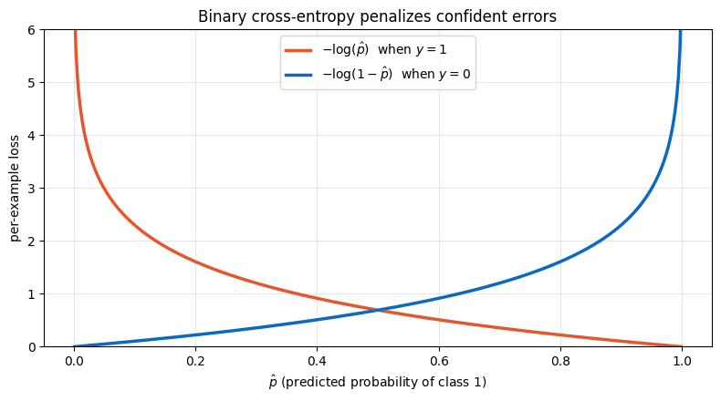
Each curve is the per-observation loss for one target value. The penalty rises sharply when the model becomes confident in the incorrect outcome.
The notebook implementation clips probabilities before applying the logarithm:
def bce(y, p_hat, eps=1e-12):
    """Return the mean binary cross-entropy."""
    p_hat = np.clip(p_hat, eps, 1 - eps)
    return -np.mean(
        y * np.log(p_hat) + (1 - y) * np.log(1 - p_hat)
    )
Clipping prevents evaluation of $\log(0)$ in this educational implementation. Production frameworks generally use a more stable formulation based directly on logits, a point we will return to below.
Why does the gradient reduce to prediction minus target?
The derivative reveals why logistic regression is both mathematically coherent and straightforward to optimize. For one observation, define
\[\ell=-\left[y\log\hat{p}+(1-y)\log(1-\hat{p})\right], \qquad \hat{p}=\sigma(z)\]
The sigmoid derivative is
\[\frac{d\hat{p}}{dz}=\hat{p}(1-\hat{p})\]
Applying the chain rule causes the probability terms to cancel:
\[\frac{d\ell}{dz}=\hat{p}-y\]
Because $z=w^\top x+b$, the dataset-level gradients are
\[\frac{\partial J}{\partial w}=\frac{1}{m}\sum_{i=1}^{m}\left(\hat{p}^{(i)}-y^{(i)}\right)x^{(i)}\]
\[\frac{\partial J}{\partial b}=\frac{1}{m}\sum_{i=1}^{m}\left(\hat{p}^{(i)}-y^{(i)}\right)\]
The residual $\hat{p}-y$ controls both expressions. A confident correct prediction produces a small residual and therefore a small update. A confident incorrect prediction produces a residual close to either $1$ or $-1$, generating a larger corrective update. The feature vector determines how that correction is distributed across the weights.
The notebook implements the equations without an optimization library:
def model(X, w, b):
    """Return the predicted probability of class 1."""
    return sigmoid(X @ w + b)


def gradient(X, y, w, b):
    """Compute the binary cross-entropy gradients."""
    residual = model(X, w, b) - y
    dw = X.T @ residual / len(y)
    db = np.mean(residual)
    return dw, db
Starting from $w=0$ and $b=0$, every observation initially receives probability $0.5$, so the mean binary cross-entropy is exactly $\log 2$. After 3,000 gradient-descent iterations with a learning rate of $0.1$, the executed output is:
BCE at w=0, b=0 (neutral 50% prediction): 0.6931
trained w = [1.610, 1.167]
trained b = -7.924
final BCE = 0.0941
accuracy  = 0.965
These values are deterministic because the dataset is generated with a fixed random seed.
How should you interpret the learned decision boundary?
With the conventional threshold of $0.5$, logistic regression predicts class 1 whenever
\[\hat{p}\geq 0.5\quad\Longleftrightarrow\quad w^\top x+b\geq 0\]
The decision boundary is therefore the line $w^\top x+b=0$. It is linear even though the probability changes nonlinearly through the sigmoid. The learned weights control the orientation of the line, and the intercept controls its position.
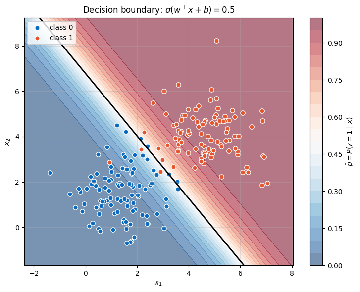
The background shows the predicted probability of class 1. The black contour marks $\hat{p}=0.5$, where the linear score is zero.
The reported accuracy of 0.965 must be interpreted carefully. It is training accuracy on the same 200 synthetic observations used for optimization. The experiment verifies the implementation and illustrates the geometry; it does not estimate performance on unseen data. A production evaluation would require a held-out test set or cross-validation, together with metrics selected for the operational objective.
Accuracy also discards probability information. Two classifiers can produce the same class labels while assigning very different levels of confidence. Log loss evaluates those probabilities, which is why the scikit-learn evaluation guide distinguishes it from threshold-based classification metrics.
What changes in a production implementation?
The NumPy version is deliberately explicit, but several additional decisions matter in a real system.
First, compute the loss from logits when possible. Evaluating a sigmoid and then taking logarithms can lose numerical precision for large positive or negative scores. PyTorch’s BCEWithLogitsLoss combines both operations and uses the log-sum-exp technique for numerical stability.
Second, use regularization and validate it. The standard LogisticRegression implementation in scikit-learn applies regularization by default and supports L1, L2, and Elastic-Net penalties. The unregularized notebook isolates the likelihood argument, but that is not automatically the best configuration for noisy or high-dimensional data.
Third, separate probability estimation from the final operating threshold. A threshold of $0.5$ is mathematically natural, but it may be inappropriate when false negatives and false positives have different costs. The threshold should be selected on validation data according to the application, while the test set remains untouched.
Finally, class imbalance changes how aggregate loss and accuracy should be interpreted. Class or observation weights may be necessary, and evaluation may need precision-recall curves, recall at a fixed precision, or application-specific expected cost. Binary cross-entropy provides the probabilistic training objective; it does not replace careful experimental design.
Takeaways
- Logistic regression models probability through the sigmoid. A linear logit is mapped from the real line to the interval $(0,1)$.
- Binary cross-entropy is a negative log-likelihood. It follows from a Bernoulli model for binary outcomes rather than from an arbitrary choice of penalty.
- Confidence changes the cost of an error. In the notebook, a wrong 99% prediction contributes
4.6052, while a correct 99% prediction contributes0.0101. - The gradient simplifies to residual times input. The key derivative is $d\ell/dz=\hat{p}-y$, which leads directly to the weight and intercept updates.
- The experiment is explanatory, not a benchmark. Its
0.965accuracy is measured on the synthetic training set and must not be read as out-of-sample performance. - Production systems should operate on logits and validate decisions. Numerical stability, regularization, class imbalance, calibration, and threshold selection remain part of the modeling problem.