

What has to change in YOLO26 when an object detector leaves a notebook and becomes part of a camera, a robot, or a system that must respond in real time?
YOLO26 is organized around that transition. Ultralytics’ 2026 model family combines an end-to-end output path without non-maximum suppression, a leaner box-regression head, and a training recipe designed to preserve accuracy while simplifying deployment. Its central contribution is not a single component. It is the coordination of architecture, label assignment, loss scheduling, and optimization.
This article examines the dual-head design, the removal of Distribution Focal Loss (DFL), Small-Target-Aware Label Assignment (STAL), Progressive Loss, and MuSGD. We will then inspect a real YOLO26n inference and separate what one successful demonstration establishes from what still needs to be measured in your own application.
Open the executed YOLO26 notebook in Google Colab
What is YOLO26?
YOLO26 is Ultralytics’ 2026 generation of computer-vision models. For object detection, the family retains the principle that made YOLO influential: the image passes through a one-stage detector that predicts classes and locations without a separate proposal-and-classification stage.
“One stage” does not mean one operation. The image still moves through many layers, feature maps, and scales. The distinction is architectural. Two-stage detectors first propose candidate regions and then classify and refine them. A YOLO detector produces its predictions through a single feature-extraction and fusion pipeline.
The version number also deserves care. YOLO is now a family of architectural lineages, not one uninterrupted sequence maintained by the same team. The original You Only Look Once paper began one lineage; universities, open-source communities, and companies later developed others. YOLO26 belongs specifically to the Ultralytics line. It is not the twenty-sixth revision of one unchanged project.
That distinction helps us evaluate the contribution on its own terms. The official YOLO26 paper presents an integrated formulation for making detector output more direct. Some mechanisms have precedents elsewhere, but their combination and controlled evaluation define the system described here.
Why reorganize the detector?
A strong COCO score does not finish the deployment problem. Between the tensors produced by a network and the decision made by an application, a pipeline may include post-processing, operators that are difficult to export, memory constraints, and large performance differences across CPUs, GPUs, and specialized accelerators.
YOLO26 addresses four connected issues:
- Duplicate boxes: dense detectors may return several high-confidence predictions for the same object, requiring a later filtering step.
- Regression-head cost: DFL represents each box edge as a discrete distribution, increasing the number of outputs.
- Small objects without eligible candidates: a tiny instance may contain no appropriate grid point during label assignment.
- A mismatch between training and inference: the branch receiving the richest supervision is not necessarily the branch used for end-to-end output.
These issues cannot be solved independently without consequences. A smaller head can reduce cost but remove a useful representation. One-to-one assignment can simplify inference but make early training harder. YOLO26 compensates for each simplification with a targeted change elsewhere in the training system.
How does the dual head remove NMS from the default path?
In a conventional dense detector, several nearby boxes can receive high confidence for one object. Non-maximum suppression, or NMS, ranks those predictions and removes redundant boxes according to their overlap. NMS is effective, but it adds post-processing and thresholds to the production pipeline.
YOLO26 trains two detection heads over shared image features:
- The one-to-many head assigns several positive candidates to each object. Its dense supervision provides an abundant learning signal.
- The one-to-one head restricts the final assignment to one prediction per object. This is the default end-to-end inference path.
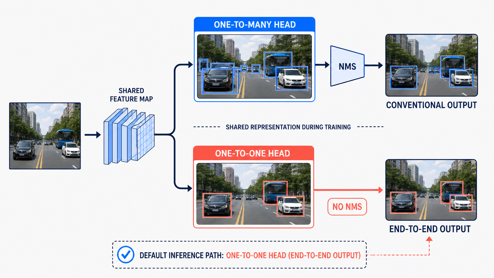
Both heads share image representations during training. At default inference, the one-to-one path sends final predictions to the application without NMS. Source: Sigmoidal, based on the Ultralytics YOLO26 paper.
An editorial selection offers a useful analogy. The one-to-many head delivers several similar photographs from which an editor chooses; the one-to-one head learns to deliver only the final selection. The first arrangement makes learning easier. The second reduces the work required after training.
With end2end=True, YOLO26 uses the one-to-one head and returns at most 300 detections per image. This does not mean NMS has disappeared from every configuration. The official documentation retains the one-to-many path, available with end2end=False during prediction, validation, or export. That path can be useful when the deployment stack runs NMS efficiently and a modest gain in average precision matters more than a simpler output path.
The choice is therefore not between a correct and an incorrect mode. It is an explicit trade-off between streamlined inference and the highest accuracy available from the conventional configuration.
Why did YOLO26 remove DFL?
A bounding box can be described by four distances from a reference point: left, top, right, and bottom. In earlier Ultralytics generations, each distance was modeled as a distribution over discrete intervals. Distribution Focal Loss converted that distribution into a continuous estimate of the edge location.
The formulation offers fine-grained localization, but it has two costs. First, the head predicts several values for every side of the box instead of one distance. Second, the discrete ruler has finite support. At higher resolutions, a large object may require a distance beyond the range represented at a particular scale.
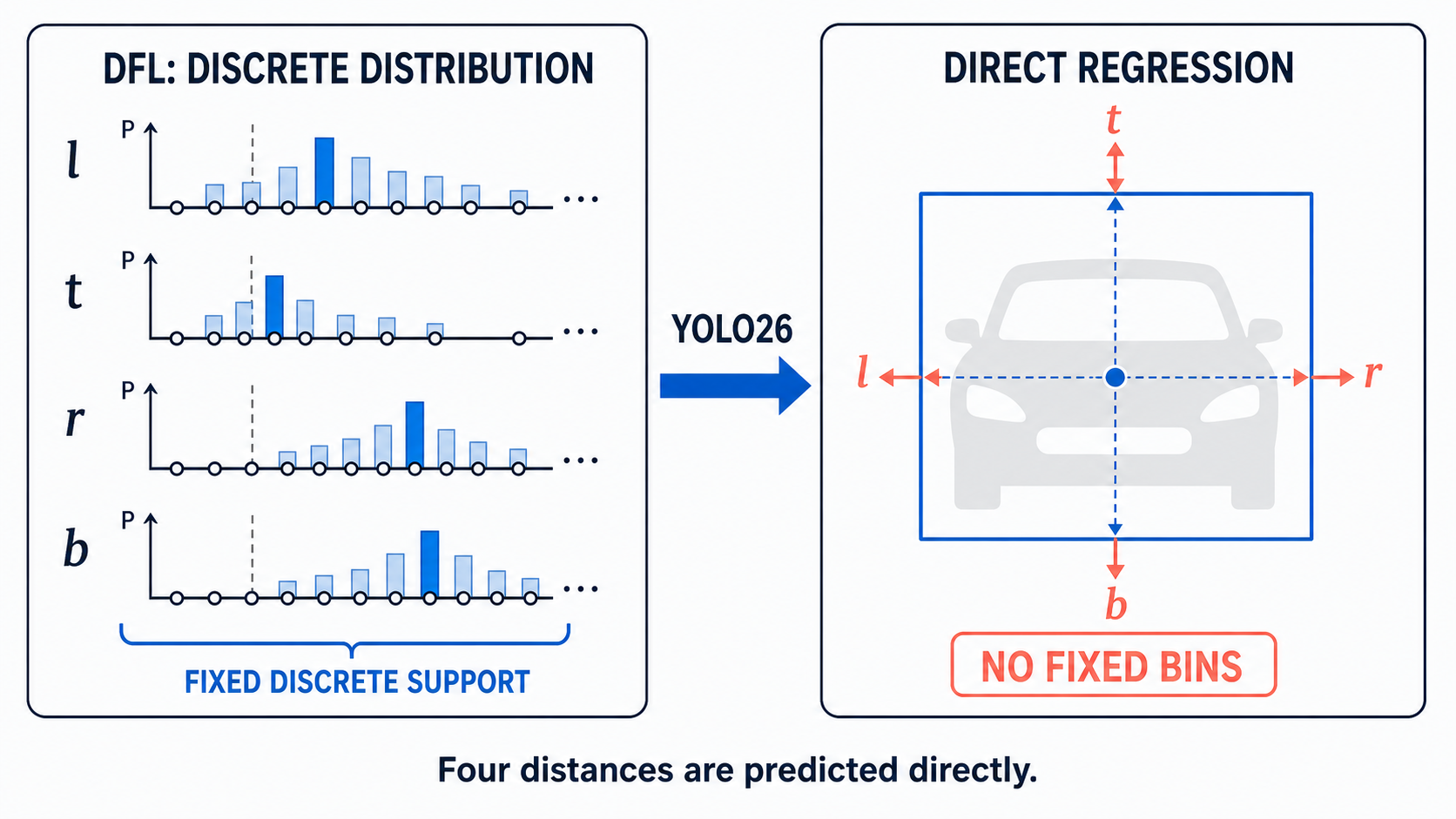
YOLO26 replaces four discrete distributions with four directly regressed distances. The change reduces output dimensionality and removes DFL’s fixed support. Source: Sigmoidal, based on the Ultralytics YOLO26 paper.
YOLO26 sets reg_max=1, removes DFL, and uses direct regression with an L1 loss. The detection head becomes smaller—especially relative to the rest of a compact model—and no longer depends on the same fixed discrete representation.
Removing DFL should not be interpreted as an accuracy improvement in isolation. In the paper’s incremental ablation, removing only DFL from the YOLO11s baseline reduced AP from 47.0 to 46.4. The revised loss, STAL, architectural refinements, and training recipe recover the quality. The simplification works as one part of a coordinated system.
How does training support a more restrictive output?
Three mechanisms complete the reorganization. STAL preserves small objects during candidate selection, Progressive Loss gradually shifts emphasis between the two heads, and MuSGD adapts the update rule to different parameter structures.
How does STAL protect small objects?
Imagine a grid of reference points over an image. A large ground-truth box contains several points that can become positive candidates. A very small box can fall between them and contain none. The object exists in the annotation, yet it may contribute no signal at that stage of training.
Small-Target-Aware Label Assignment introduces a minimum auxiliary region for candidate selection. It increases the chance that a small instance receives candidates, but it does not enlarge the true box used for the final assignment and regression target. The model is not taught that the object is larger; it is simply prevented from discarding the object before learning begins.
In the authors’ ablation, STAL with a reference size of 16 raised small-object AP from 29.0 to 29.6 and overall AP from 46.6 to 46.8. This is a specific measured result, not a universal solution to every scale problem. Other reference sizes did not reproduce the same gain.
How does Progressive Loss shift responsibility?
The one-to-many head learns more easily at the beginning because it receives many positive examples. The one-to-one head faces a more restrictive task, but it is the branch used for end-to-end deployment. Giving both branches the same importance throughout training would preserve a mismatch between the best-supervised branch and the deployed branch.
Progressive Loss implements a curriculum. Early training emphasizes dense supervision; its weighting then shifts linearly toward the one-to-one head. The final branch is never switched off—it participates from the first epoch and progressively assumes the central role. Training begins with abundant signals and ends aligned with the inference regime.
What changes with MuSGD?
Convolution weights are matrices or higher-dimensional tensors, while biases and normalization scales are one-dimensional parameters. MuSGD separates these groups: it applies a weighted combination of Muon and SGD updates to structural weights while retaining conventional SGD for simpler parameters.
In the paper’s controlled detection experiment, MuSGD reached 47.4 mAP after 500 epochs, compared with 47.0 after 600 epochs for the SGD reference. That is a 16.7% reduction in epochs under the evaluated recipe—not a guarantee that every dataset will converge on the same schedule.
What do the benchmarks actually show?
The detection family has five scales, from YOLO26n to YOLO26x. The figures below were published for 640-pixel images on COCO val2017:
| Model | mAP 50–95 | End-to-end mAP 50–95 | CPU ONNX | T4 TensorRT | Parameters |
|---|---|---|---|---|---|
| YOLO26n | 40.9 | 40.1 | 38.9 ms | 1.7 ms | 2.4 M |
| YOLO26s | 48.6 | 47.8 | 87.2 ms | 2.5 ms | 9.5 M |
| YOLO26m | 53.1 | 52.5 | 220.0 ms | 4.7 ms | 20.4 M |
| YOLO26l | 55.0 | 54.4 | 286.2 ms | 6.2 ms | 24.8 M |
| YOLO26x | 57.5 | 56.9 | 525.8 ms | 11.8 ms | 55.7 M |
Source: Ultralytics YOLO26 documentation. CPU latency uses ONNX; GPU latency uses TensorRT on an Amazon EC2 P4d instance, batch size 1. Parameter counts refer to the fused deployment model after model.fuse(), which removes the auxiliary one-to-many head.
The benchmark and ablations come from the organization that develops the model. They provide useful technical evidence and reproducible conditions, but they do not replace independent evaluation or a test in the target domain.
Three observations matter. First, the end-to-end path remains 0.6 to 0.8 AP below the conventional result in this table. Second, latency changes sharply with model scale, so a comparison that says only “YOLO26” without naming the variant is incomplete. Third, none of these figures transfers automatically to another processor, backend, image size, or batch size.
Ultralytics also reports YOLO26n as up to 43% faster than YOLO11n on CPU ONNX under its documented protocol. The phrase up to is essential. For a production deployment, measure the complete pipeline: image decoding, preprocessing, inference, memory transfer, and consumption of the predictions.
How can you test YOLO26 in Python?
The companion notebook pins a reproducible dependency set, validates Ultralytics’ canonical bus.jpg image by checksum, and loads the compact yolo26n.pt checkpoint. The core inference requires four lines:
from ultralytics import YOLO

model = YOLO("yolo26n.pt")
result = model("bus.jpg")[0]
result.save(filename="yolo26_result.jpg")
The constructor downloads the official weights on the first run. The model returns a Results object containing boxes, classes, and confidence scores; save renders those predictions over the source image.
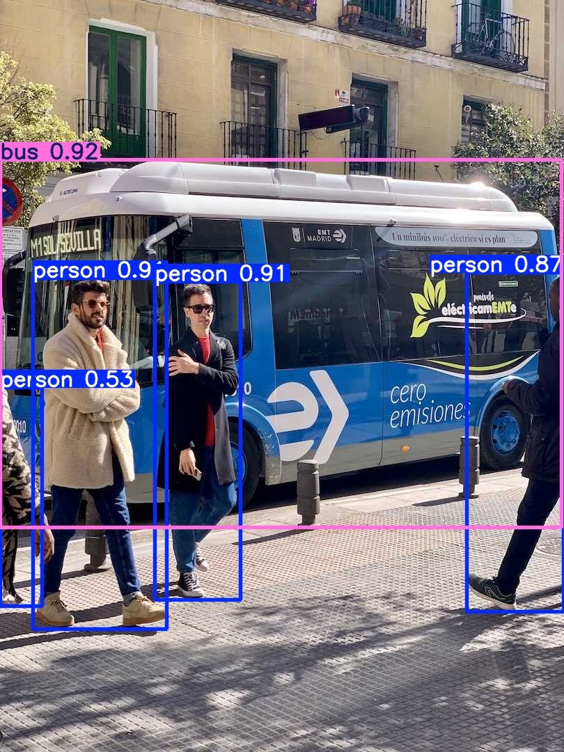
Validated with Ultralytics 8.4.118 and end2end=True: five detections—one bus and four people. Original image: Ultralytics; inference and rendering: Sigmoidal.
The executed notebook confirmed that the model uses end2end=True by default. It returned five detections: one bus and four people. The final table reports every class, confidence score, and coordinate instead of relying only on the rendered image. The recorded confidences were 92.4% for the bus and 91.3%, 90.5%, 87.0%, and 53.5% for the four people.
This run establishes that the official integration works and produces a coherent output. It does not establish generalization. One canonical image says nothing about low light, severe occlusion, aerial cameras, industrial defects, or classes that do not exist in COCO.
How should you evaluate YOLO26 in your domain?
A responsible evaluation begins with representative data. Build an annotated set covering lighting, distance, angle, object density, and expected failure cases. Measure precision, recall, and mAP per class, giving special attention to errors with the highest operational cost.
Record latency and memory use on the target hardware at the same time. A datacenter GPU may reverse a result observed on an embedded CPU; a backend with an efficient NMS implementation may make the conventional head attractive; a particular export path may introduce extra operators or conversions.
Licensing is also part of deployment. Ultralytics offers its software under AGPL-3.0 and an Enterprise license. Before embedding the model in a proprietary product or commercial service, verify which terms apply to the way the system is distributed and operated.
The principle applies to every YOLO generation. Our YOLOv9 object-detection tutorial makes the same distinction: a demonstration validates the technical path; an evaluation on your own data determines whether the model fits the application.
Which tasks does the YOLO26 family support?
The current ecosystem includes models for object detection, instance segmentation, semantic segmentation, depth estimation, image classification, pose estimation, and oriented bounding boxes. YOLOE extends the ecosystem toward open-vocabulary detection. These variants share the library’s training and deployment experience, but they do not use identical heads and loss functions.
Every mechanism and inference number discussed in this article refers to standard object detection. Conclusions from the detection table should not be transferred automatically to segmentation, pose, or depth estimation.
What has been announced about YOLO27?
The official Ultralytics roadmap lists YOLO27 for Ultralytics YOLO Vision in September 2026. The stated direction is to extend the family toward vision-language systems, with a YOLO front end feeding a language-model layer in a proposed YOLO-VLM.
As of this publication, that is a roadmap announcement, not a released model. There are not yet official weights and results sufficient for a reproducible YOLO27-versus-YOLO26 comparison. Vision-language capability should therefore be described as an announced direction until the release can be tested.
Takeaways
- YOLO26 prioritizes a more direct production output: the one-to-one head enables end-to-end inference without NMS by default.
- The conventional path remains available:
end2end=Falseuses the one-to-many branch with NMS when maximum AP is the priority. - Removing DFL simplifies box regression: four direct distances replace discrete distributions, but the rest of the recipe is needed to recover quality.
- STAL prevents empty candidate sets for small targets: the selection region grows while the true box stays unchanged.
- Progressive Loss aligns training with deployment: supervision shifts gradually from the dense branch toward the inference head.
- MuSGD adapts updates to parameter structure: its published gains remain specific to the evaluated recipe.
- A demonstration is not validation: your data, backend, and hardware remain the decisive test.