What is Sampling and Quantization in Image Processing

Have you ever stopped to think about what happens between the moment light enters a camera lens, is focused at the focal point, passes through the Bayer filter, hits the sensor… and then that electromagnetic wave transforms into an array of numbers representing the captured image?

How can a continuous wave from the real world turn into a matrix with values between 0 and 255?

In this article, I will show you the basic principle behind the formation of digital images. We will understand how a digital image can be formed through two fundamental processes: sampling and quantization. The complete source code with Python examples is available below.

Sampling and Quantization

Just as for Aristotle, motion is the transition from potentiality to actuality, the creation of a digital image represents the realization of a continuous visual potential (captured by light) into a finite set of discrete data through sampling and quantization.

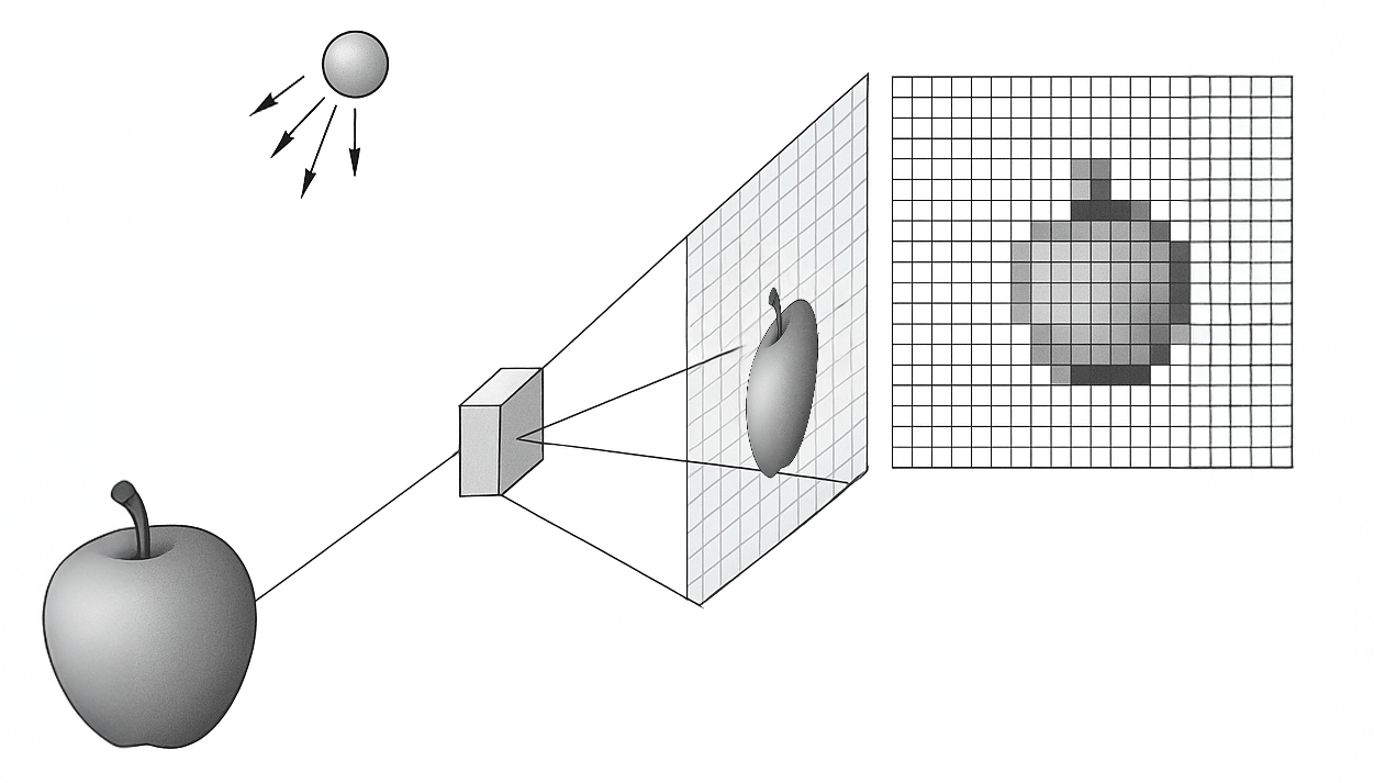
Imagine a photograph as an infinite painting, where each point in the image plane has a light intensity. This intensity is described by a continuous function defined as:

$f: \mathbb{R}^2 \rightarrow \mathbb{R},$

where $f(x, y)$ represents the grayscale level (or brightness) at the point $(x, y)$ . In the real world, $x$ and $y$ can take any real value, but a computer requires a finite representation: a grid of discrete points.

Sampling: Discretization of the image in the spatial domain $(x, y)$

Spatial sampling is the process of selecting values of this function on a regular grid, defined by intervals $\Delta x$ and $\Delta y$ . The result is a matrix $M = (m_{ij})$ of dimensions $W \times H$ , where $W$ is the width and $H$ is the height in pixels. Each element of the matrix is given by:

$m_{ij} = f(x_0 + i \cdot \Delta x, y_0 + j \cdot \Delta y)$

Think of it as placing a checkered screen over the painting: each square (pixel) captures the average value of $f$ at that point.

The spatial resolution depends on the density of this grid, measured in pixels per unit of distance (such as DPI, or dots per inch). Smaller values of $\Delta x$ and $\Delta y$ mean more pixels, capturing finer details, like the outlines of a leaf in a photograph.

$\text{Continuous image: } f(x, y) \quad \rightarrow \quad \text{Digital image: } \begin{bmatrix} m_{00} & m_{01} & \cdots & m_{0, W-1} \\ m_{10} & m_{11} & \cdots & m_{1, W-1} \\ \vdots & \vdots & \ddots & \vdots \\ m_{H-1, 0} & m_{H-1, 1} & \cdots & m_{H-1, W-1} \end{bmatrix}.$

For example, a Full HD image ( $1920 \times 1080$ pixels) has higher spatial resolution than a VGA image ( $640 \times 480$ pixels), assuming the same physical area. Spatial sampling can be visualized as the transformation of a continuous function into a discrete matrix, as shown above.

Quantization: Discretization of intensity levels

With the grid of points defined, the next step is to discretize the intensity values. In the real world, these values are continuous, but a computer requires a finite number of levels. This process, called intensity quantization, is performed by a quantization function:

$q: \mathbb{R} \rightarrow \{0, 1, \ldots, L-1\},$

where $L$ is the number of intensity levels. For grayscale images, it is common to use 1 byte (8 bits) per pixel, resulting in $L = 2^8 = 256$ levels, with 0 representing black and 255 representing white.

Imagine intensity as the height of a wave at each pixel. Quantization is like measuring that height with a ruler that has only $L$ markings. The function $q$ maps each real value to the nearest discrete level, creating a staircase-like representation. Thus, the pixel value at position $(i, j)$ is:

$m_{ij} = q(f(x_0 + i \cdot \Delta x, y_0 + j \cdot \Delta y)).$

Intensity Resolution

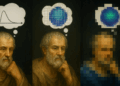
The intensity resolution, determined by $L$ , affects visual quality. With $L = 256$ (8 bits), brightness transitions are smooth, ideal for common photos. However, with $L = 16$ (4 bits), artifacts like the “banding” effect appear, where color bands become visible.

In medical applications, such as tomography, 10 to 12 bits ( $L = 1024$ or $4096$ ) are used for greater fidelity.

For numerical processing, values can be normalized to the interval $[0, 1]$ by an affine transformation $f \leftarrow a f + b$ , and requantized for storage.

Discrete Structure and Computational Implications

Spatial sampling and intensity quantization convert a continuous image into a matrix of integers, where each $m_{ij}$ represents the intensity of a pixel.

This discrete structure is the foundation of digital processing and imposes practical limitations. The space required to store an image is given by:

$b = W \cdot H \cdot k, \quad \text{with } k = \log_2(L).$

For example, for a Full HD image ( $1920 \times 1080$ ) with $L = 256$ ( $k = 8$ bits), we have:

$b = 1920 \cdot 1080 \cdot 8 = 16,588,800 \text{ bits} \approx 2 \text{ MB}.$

This justifies the use of compression (like JPEG), which reduces the final size by exploiting redundant patterns without significant visual loss.

Both spatial resolution ( $W \times H$ ) and intensity ( $L$ ) affect computer vision algorithms. More pixels increase detail and computational cost; more bits per pixel improve accuracy but require more memory.

Sampling and Quantization in Practice with Python

Now, let’s explore two practical examples to understand how continuous signals are transformed into digital representations. First, we’ll simulate a one-dimensional (1D) signal, like the sound of a musical instrument. Then, we’ll apply the same concepts to a real grayscale image.

Example 1: Sampling and Quantization of a 1D Signal

Imagine you’re recording the sound of a guitar. The vibration of the strings creates a continuous sound wave, but to turn it into a digital file, we need to sample in time and quantize the amplitude.

Let’s simulate this with a synthetic signal—a combination of sines that mimics complex variations, like a musical note. We’ll divide this example into three parts: signal generation, sampling, and quantization.

Part 1: Generating the Continuous Signal

First, we create an analog signal by combining three sines with different frequencies. This simulates a complex signal, like a sound wave or a light pattern.

# Importing necessary libraries
import numpy as np
import matplotlib.pyplot as plt

# Generating a continuous signal (combination of sines)
x = np.linspace(0, 4*np.pi, 1000)
y = np.sin(x) + 0.3 * np.sin(3*x) + 0.2 * np.cos(7*x)

What’s happening here?

We use np.linspace to create 1000 points between $0$ and $4\pi$ , “simulating” the continuous domain (like time).
The signal $y$ is a sum of sines ( $\sin(x) + 0{.}3\sin(3x) + 0{.}2\cos(7x)$ ), creating smooth and abrupt variations, like in a real signal.
The graph shows the continuous wave, which is what a sensor (like a microphone) would capture before digitization.

Part 2: Sampling the Signal

Now, we sample the signal at regular intervals, simulating what a sensor does when capturing values at discrete points.

# Sampling: discretizing the continuous domain
sample_factor = 20
x_sampled = x[::sample_factor]
y_sampled = y[::sample_factor]

What’s happening here?

The sample_factor = 20 reduces the signal to 1/20 of the original points, taking 1 point every 20.
x[::sample_factor] and y[::sample_factor] select regularly spaced points, simulating spatial or temporal sampling.
The graph shows the samples (red points) over the continuous signal, highlighting the domain discretization.

Part 3: Quantizing the Sampled Signal

Finally, we quantize the sampled values, limiting the amplitude to 8 discrete levels, as an analog-to-digital converter would do.

# Quantization: reducing amplitude resolution
num_levels = 8
y_min, y_max = y.min(), y.max()
step = (y_max - y_min) / num_levels
y_quantized = np.floor((y_sampled - y_min) / step) * step + y_min

# Plotting the signal with sampling and quantization
plt.figure(figsize=(10, 4))
plt.plot(x, y, label='Continuous Signal', alpha=0.75, color='blue')
markerline, stemlines, baseline = plt.stem(x_sampled, y_sampled,
                                          linefmt='r-', markerfmt='ro', basefmt=' ',
                                          label='Samples')
plt.setp(markerline, alpha=0.2)
plt.setp(stemlines, alpha=0.2)

# Horizontal quantization lines
for i in range(num_levels + 1):
    y_line = y_min + i * step
    plt.axhline(y_line, color='gray', linestyle='--', linewidth=0.5, alpha=0.6)

# Vertical sampling lines
for x_tick in x_sampled:
    plt.axvline(x_tick, color='gray', linestyle='--', linewidth=0.5, alpha=0.6)

# Quantization boxes with filling
delta_x = (x[1] - x[0]) * sample_factor
for xi, yi in zip(x_sampled, y_quantized):
    plt.gca().add_patch(plt.Rectangle(
        (xi - delta_x / 2, yi),
        width=delta_x,
        height=step,
        edgecolor='black',
        facecolor='lightgreen',
        linewidth=1.5,
        alpha=0.85
    ))

# Quantized points
plt.scatter(x_sampled, y_quantized, color='green', label='Quantized')
plt.title("Sampled and Quantized Signal (8 Levels felici)")
plt.xlabel("Time")
plt.ylabel("Amplitude")
plt.legend()
plt.grid(False)
plt.tight_layout()
plt.show()

What’s happening here?

We calculate the quantization interval (step) by dividing the total amplitude (y_max - y_min) by num_levels = 8.
The np.floor function maps each sampled value to the nearest quantized level.
Green rectangles highlight the quantization “boxes,” showing how continuous values are approximated by discrete levels.
The final graph combines the continuous signal, samples, and quantized values, illustrating the loss of fidelity.

Practical tip: Try changing sample_factor to 10 (more samples) or num_levels to 4 (fewer levels) and observe how the signal becomes more or less faithful to the original.

Example 2: Sampling and Quantization of a Real Image

Now, let’s apply sampling and quantization to a real image, like a photo you’d take with your phone. Here, spatial sampling defines the resolution (number of pixels), and intensity quantization determines the grayscale tones.

Part 1: Loading the Grayscale Image

First, we load an image and convert it to grayscale, turning it into a NumPy matrix.

# Importing necessary libraries
import numpy as np
import matplotlib.pyplot as plt
from PIL import Image
from pathlib import Path

# Base path for images
NOTEBOOK_DIR = Path.cwd()
IMAGE_DIR = NOTEBOOK_DIR.parent / "images"

# Loading grayscale image
img = Image.open(IMAGE_DIR / 'hexapod.jpg').convert('L')
img_np = np.array(img)

# Displaying original image
plt.figure(figsize=(6, 4))
plt.imshow(img_np, cmap='gray')
plt.title("Original Grayscale Image")
plt.axis('off')
plt.show()

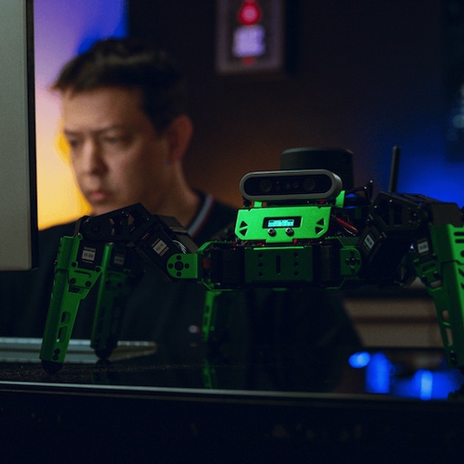
**My photo with the hexapod, used to demonstrate the concepts of sampling and quantization in digital images.**

What’s happening here?

We use PIL.Image.open to load the image hexapod.jpg and .convert('L') to transform it into grayscale (values from 0 to 255).
We convert the image into a NumPy matrix (img_np) for numerical manipulation.
The graph shows the original image, representing a continuous scene before manipulation.

Part 2: Spatial Sampling of the Image

We reduce the image’s resolution, simulating a camera with fewer pixels.

# Spatial sampling with factor 4
sampling_factor = 4
img_sampled = img_np[::sampling_factor, ::sampling_factor]

# Displaying sampled image
plt.figure(figsize=(6, 4))
plt.imshow(img_sampled, cmap='gray', interpolation='nearest')
plt.title("Image with Spatial Sampling (Factor 4)")
plt.axis('off')
plt.show()

What’s happening here?

The sampling_factor = 4 reduces the resolution, taking 1 pixel every 4 in both dimensions (width and height).
img_np[::sampling_factor, ::sampling_factor] selects a submatrix, reducing the number of pixels.
The result is a more “pixelated” image with fewer details, as if captured by a low-resolution camera.

Part 3: Intensity Quantization of the Image

Now, we quantize the values of the sampled image, reducing the grayscale tones to 8 and then to 2 levels.

# Uniform quantization function
def quantize_image(image, levels):
    image_min = image.min()
    image_max = image.max()
    step = (image_max - image_min) / levels
    return np.floor((image - image_min) / step) * step + image_min

# Quantizing the sampled image (8 levels)
quantization_levels = 8
img_quantized_8 = quantize_image(img_sampled, quantization_levels)

# Displaying sampled and quantized image (8 levels)
plt.figure(figsize=(6, 4))
plt.imshow(img_quantized_8, cmap='gray', interpolation='nearest')
plt.title("Sampled + Quantized Image (8 Levels)")
plt.axis('off')
plt.show()

# Quantizing the sampled image (2 levels)
quantization_levels = 2
img_quantized_2 = quantize_image(img_sampled, quantization_levels)

# Displaying sampled and quantized image (2 levels)
plt.figure(figsize=(6, 4))
plt.imshow(img_quantized_2, cmap='gray', interpolation='nearest')
plt.title("Sampled + Quantized Image (2 Levels)")
plt.axis('off')
plt.show()

What’s happening here?

The quantize_image function maps intensity values to levels discrete values, calculating the interval (step) and rounding with np.floor.
With 8 levels, the image retains some fidelity but loses smooth tone transitions.
With 2 levels, the image becomes binary (black and white), showing the extreme effect of quantization.
The graphs show how reducing levels creates visual artifacts, like “banding.”

Practical tip: Try changing sampling_factor to 8 or quantization_levels to 16 and see how the image gains or loses quality.

Takeaways

Spatial sampling transforms a continuous image into a pixel matrix, defined by a grid of intervals $\Delta x$ and $\Delta y$ . The density of this grid (spatial resolution) determines the amount of detail captured.
Intensity quantization reduces continuous brightness values to a finite set of levels ( $L$ ). A lower $L$ (like 2 or 8 levels) causes loss of detail but can be useful in specific applications, like binarization.
The combination of sampling and quantization defines the structure of a digital image, directly impacting file size ( $b = W \cdot H \cdot \log_2(L)$ ) and the performance of computer vision algorithms.
In practical applications, like digital cameras or medical imaging, balancing spatial and intensity resolution is crucial for optimizing quality and computational efficiency.
The Python examples illustrate how sampling and quantization visually alter an image, from preserving details with 8 levels to extreme simplification with 2 levels.