Matrix Transformations and Coordinate Systems with Python

In the fascinating realm of camera projection and computer vision, understanding matrix transformations and coordinate systems is essential for accurately converting 3D objects into 2D images. This process, widely utilized in applications like video games, virtual reality, and augmented reality, enables realistic image rendering by mapping 3D points in the world to 2D points on an image plane.

In this tutorial, we’ll explore the intricacies of matrix transformations and coordinate systems, focusing on the imaging geometry of the camera, image, and world coordinates. We will include a Python implementation to help illustrate these concepts, focusing on how to manipulate the camera and obtain its coordinates.

Geometry of Image Formation

To comprehend the formation of an image from a 3D point in space, we must understand the process from the perspective of geometry and linear algebra. Essentially, we need to project a 3D point onto a 2D image plane using a process called perspective projection.

This involves taking into account three critical components: the World Coordinate System, the Camera Coordinate System, and the Image Plane. To transform from World to Pixel coordinates, we perform the following three steps:

Transform the world point $(X_W, Y_W, Z_W)$ with optical center $W$ to a new coordinate system with the camera’s optical center $C$ as the $(0, 0, 0)$ origin. This is done using a rigid body transformation, consisting of rotation $(R)$ and translation $(t)$ .
Project the camera point $(X_C, Y_C, Z_C)$ onto the optical sensor, creating new coordinates $(x, y, z)$ in the same coordinate system. This is achieved using the camera’s intrinsic parameter matrix $K$ . The optical sensor is often referred to as the “image plane” or “image frame.”
Normalize $(x, y, z)$ to pixel coordinates $(u, v)$ by dividing by $z$ and adjusting the origin of the image.

By understanding and applying these steps, we can effectively convert a 3D point from the World Coordinate System to pixel coordinates on an image, which is essential in the field of computer vision and image formation.

World Coordinate System

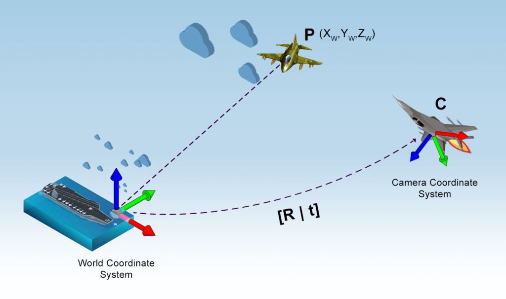
Imagine you’re a top gun pilot, Maverick, engaging in a high-stakes dogfight against an enemy aircraft. To describe the position of objects in the airspace, you need to establish a coordinate system for the 3D world in which you’re flying.

This process involves two key components:

Origin: We can arbitrarily select any point in the 3D world as the origin, such as the navy aircraft carrier, represented by coordinates $(0, 0, 0)$ .
X, Y, Z axes: Next, we define the X, Y, and Z axes based on a fixed reference, such as the aircraft carrier’s longitudinal axis, lateral axis, and the vertical line pointing towards the sky from the top guns.

With our coordinate system in place, we can determine the 3D coordinates of any point $P$ within the airspace by measuring its distance from the origin along the X, Y, and Z axes. This coordinate system is known as the World Coordinate System.

Camera Coordinate System

Now, imagine Maverick tearing through the skies beyond enemy lines in his F-18 Super Hornet, skillfully navigating all axes to engage and lock onto a target aircraft. Maverick’s objective is to establish a line of sight with the enemy aircraft, making it appear on his Heads-Up Display (HUD) screen.

For educational purposes, let’s consider the aircraft and its pilot as a camera. The enemy aircraft’s image must be captured by this camera, so we’re interested in the 3D coordinate system attached to it, known as the camera coordinate system. In such a scenario, we need to find the relationship between the 3D world coordinates and the 3D camera coordinates.

If we were to place the camera at the origin of the world coordinates and align its X, Y, and Z axes with the world’s axes, the two coordinate systems would be identical. However, that is an impractical constraint. We want the camera to be anywhere in the world and able to look in any direction. In this case, we need to find the relationship between the 3D world and 3D camera ‘Maverick’ coordinates.

Camera Pixel Coordinates on the left vs World Coordinates on the right. Fonte: Intel RealSense

Assume Maverick’s aircraft is at an arbitrary location $(t_X, t_Y, t_Z)$ in the airspace. The camera coordinate is translated by $(t_X, t_Y, t_Z)$ with respect to the world coordinates. Additionally, the aircraft can look in any direction, meaning it is rotated concerning the world coordinate system.

In 3D, rotation is captured using three parameters—yaw, pitch, and roll. These can also be represented as an axis in 3D (two parameters) and an angular rotation about that axis (one parameter). For mathematical manipulation, it’s often more convenient to encode rotation as a 3×3 matrix. Although a 3×3 matrix has nine elements, a rotation matrix has only three degrees of freedom due to the constraints of rotation.

With this information, we can establish the relationship between the World Coordinate System and the Camera Coordinate System using a rotation matrix R and a 3-element translation vector $t$ .

This means that point P, which had coordinate values $(X_W, Y_W, Z_W)$ in the world coordinates, will have different coordinate values $(X_C, Y_C, Z_C)$ in the camera coordinate system. The two coordinate values are related by the following equation:

$\begin{bmatrix} X_C \\ Y_C \\ Z_C \end{bmatrix} = \mathbf{R} \begin{bmatrix} X_W \\ Y_W \\ Z_W \end{bmatrix} + \mathbf{t}$

By representing rotation as a matrix, we can simplify rotation with matrix multiplication instead of tedious symbol manipulation required in other representations like yaw, pitch, and roll. This should help you appreciate why we represent rotations as a matrix. Sometimes the expression above is written in a more compact form. The 3×1 translation vector is appended as a column at the end of the 3×3 rotation matrix to obtain a 3×4 matrix called the Extrinsic Matrix:

$\begin{bmatrix} u \\ v \\ 1 \end{bmatrix} = P \begin{bmatrix} X_C \\ Y_C \\ Z_C \\ 1 \end{bmatrix}$

where the camera projection matrix P is given by:

$P = K \begin{bmatrix} R \ | \ t \end{bmatrix}$

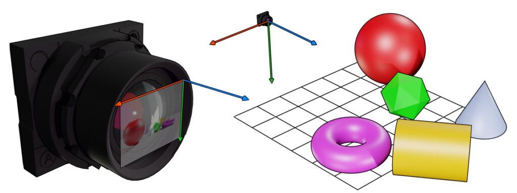
Image Coordinate System: Locking on Target

In this high-stakes dogfight, Maverick must bring the enemy aircraft into his Head-Up Display (HUD) to lock onto the target and establish a firing solution. Analogously, we need to project a 3D point from the camera coordinate system onto the image plane. The image plane, a 2D plane representing the camera’s field of view, is where our 3D world is projected to form a 2D image.

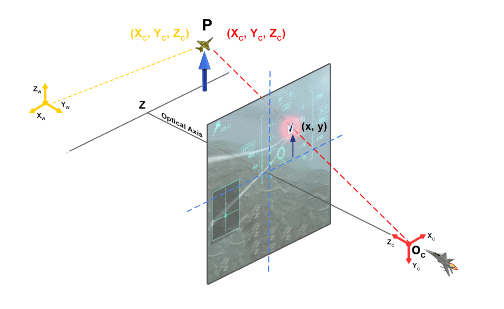
The projection of point P (enemy aircraft) onto the image plane (HUD).

The Image Coordinate System has its origin at the bottom-left corner of the image plane, with the X and Y axes extending to the right and up, respectively. Typically, the units of measurement are in pixels, starting at the origin (0, 0) and reaching the maximum coordinates according to the image width and height.

To project a 3D point from the camera coordinate system onto the image plane, we first need to establish the relationship between the camera’s intrinsic parameters and the Image Coordinate System. The intrinsic parameters include the focal length (f) and the principal point $(u_0, v_0)$ , which represents the image plane’s center.

The camera’s intrinsic parameter matrix, denoted as K, is defined as:

$K = \begin{bmatrix} f & 0 & u_0 \\ 0 & f & v_0 \\ 0 & 0 & 1 \end{bmatrix}$

Now that we have the intrinsic parameter matrix, we can project a 3D point from the camera coordinate system $(X_C, Y_C, Z_C)$ onto the image plane using the following equation:

$\begin{bmatrix} x \\ y \\ z \end{bmatrix} = K \begin{bmatrix} X_C \\ Y_C \\ Z_C \end{bmatrix}$

Finally, we normalize the projected point (x, y, z) to obtain the corresponding pixel coordinates $(u, v)$ on the image plane:

$u = \frac{x}{z} \quad \text{and} \quad v = \frac{y}{z}$

Putting It All Together

As Maverick maneuvers his F-18 Super Hornet and locks onto the enemy aircraft, he can now project the target’s position onto his HUD. This analogy helps us understand the process of projecting a 3D point onto a 2D plane in the field of computer vision.

In a more general context, we have successfully projected a 3D point from the world coordinate system to the image coordinate system, transforming it into a 2D image. By understanding and applying the concepts of the World Coordinate System, the Camera Coordinate System, and the Image Coordinate System, we can effectively convert 3D points into pixel coordinates on an image. This process is crucial for various applications in computer graphics, such as video games, virtual reality, and augmented reality.

Python implementation

In the “Python implementation” section, we will explore how to manipulate camera position and orientation in a 3D space using Python. We will use the concepts of camera projection and imaging geometry to create a Python implementation that demonstrates the relationship between the world and camera coordinate systems.

import numpy as np
import matplotlib.pyplot as plt
from mpl_toolkits.mplot3d import Axes3D
from scipy.linalg import expm

class Camera:
    def __init__(self, P):
        self.P = P
        self.K = None
        self.R = None
        self.t = None
        self.c = None

    def translate(self, translation_vector):
        T = np.eye(4)
        T[:3, 3] = translation_vector
        self.P = np.dot(self.P, T)

    def rotate(self, rotation_vector):
        R = rotation_matrix(rotation_vector)
        self.P = np.dot(self.P, R)

    def position(self):
        return self.P[:3, 3]

def rotation_matrix(a):
    R = np.eye(4)
    R[:3, :3] = expm(np.array([[0, -a[2], a[1]], [a[2], 0, -a[0]], [-a[1], a[0], 0]]))
    return R

This particular code block illustrates a Python implementation of a Camera class that can be used to perform translations and rotations on a 3D projection matrix. The Camera class has methods to translate and rotate the camera, and a position method that returns the position of the camera. The rotation_matrix function is used to create a rotation matrix from a rotation vector, which is then used to update the projection matrix. The numpyand scipy libraries are used to perform matrix operations and calculate the exponential of a matrix, respectively. The matplotlib library is used to visualize the 3D projection.

def draw_axis(ax, position, label, color):
    x_arrow = np.array([1, 0, 0])
    y_arrow = np.array([0, 1, 0])
    z_arrow = np.array([0, 0, 1])
    ax.quiver(*position, *x_arrow, color=color, arrow_length_ratio=0.1)
    ax.quiver(*position, *y_arrow, color=color, arrow_length_ratio=0.1)
    ax.quiver(*position, *z_arrow, color=color, arrow_length_ratio=0.1)
    ax.text(*(position + x_arrow), f"{label}_x")
    ax.text(*(position + y_arrow), f"{label}_y")
    ax.text(*(position + z_arrow), f"{label}_z")

def plot_world_and_camera(world_coordinates, camera):
    fig = plt.figure(figsize=(10, 10))
    ax = fig.add_subplot(111, projection='3d')

    world_x, world_y, world_z = zip(world_coordinates)
    ax.scatter(world_x, world_y, world_z, c='b', marker='o', label='World Coordinates', s=54)

    camera_x, camera_y, camera_z = camera.position()
    ax.scatter(camera_x, camera_y, camera_z, c='r', marker='^', label='Camera Position', s=54)

    draw_axis(ax, camera.position(), "C", color="red")
    draw_axis(ax, world_origin, "W", color="blue")

    ax.set_xlabel('X')
    ax.set_ylabel('Y')
    ax.set_zlabel('Z')
    ax.set_xlim(-3, 3)
    ax.set_ylim(-3, 3)
    ax.set_zlim(-3, 3)
    ax.legend()
    plt.show()

This code snippet demonstrates the plot_world_and_camera function that is used to plot the world coordinates and camera position in a 3D space. The function takes in the world_coordinates and camera objects as arguments and creates a 3D scatter plot using the matplotlib library. The draw_axis function is used to draw the x, y, and z axes for both the world and camera coordinate systems. The camera.position() method is used to get the position of the camera in the world coordinate system. The ax.set_xlabel, ax.set_ylabel, and ax.set_zlabel methods are used to label the x, y, and z axes, respectively. Finally, the ax.legend() and plt.show() methods are used to display the legend and plot, respectively.

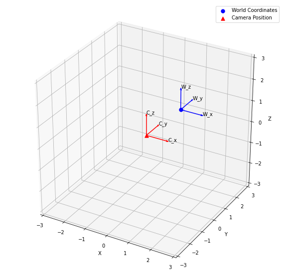
world_origin = (1, 1, 1)

# Set up Camera
P = np.hstack((np.eye(3), np.array([[0], [0], [0]])))
cam = Camera(P)

# Plot the World and Camera Coordinate Systems
plot_world_and_camera(world_origin, cam)

As demonstrated in the above code snippet, the world_origin variable is initialized to the coordinates (1, 1, 1). The P variable is initialized to a 3×4 identity matrix, which represents the camera projection matrix. The Cameraclass is then initialized with the P matrix. Finally, the plot_world_and_camera function is called with the world_origin and cam objects as arguments to plot the world coordinates and camera position in a 3D space.

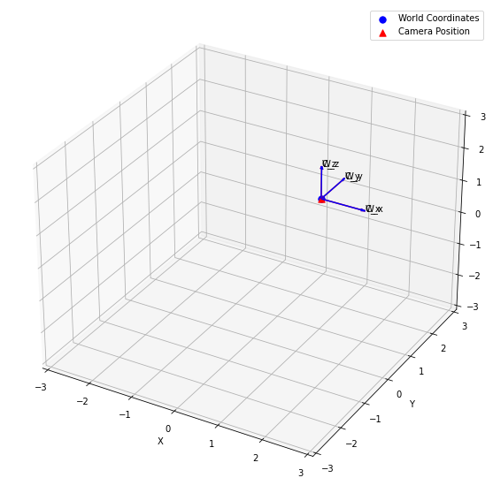
Now we will move the camera by applying a translation and rotation. We initialize the translation_vector to [1, 1, 1] and the rotation_axis to [0, 0, 1]. We then set the rotation_angle to np.pi / 4. Next, we create a rotation_vector by multiplying the rotation_axis by the rotation_angle. Finally, we apply the translation and rotation to the camera using the translate and rotate methods, respectively. After that, we plot the updated world and camera coordinate systems using the plot_world_and_camera function.

# Move the Camera
translation_vector = np.array([1, 1, 1])
rotation_axis = np.array([0, 0, 1])
rotation_angle = np.radians(45)
rotation_vector = rotation_axis * rotation_angle
cam.translate(translation_vector)
cam.rotate(rotation_vector)

## Plot the World and Camera Coordinate Systems after moving the Camera
plot_world_and_camera(world_origin, cam)

By executing this code snippet, you will be able to visualize the updated positions of the camera and world coordinate systems after applying the translation and rotation to the camera. This will help you understand how the camera projection matrix changes as the camera moves in the 3D world.

In conclusion, we have demonstrated how to manipulate the camera position and orientation in a 3D space using Python by implementing the camera projection and imaging geometry concepts. We have also provided a Python implementation of a Camera class, which can be used to perform translations and rotations on a 3D projection matrix. By understanding and applying these concepts, you will be able to create and manipulate virtual cameras in 3D space, which is crucial for various applications in computer graphics, such as video games, virtual reality, and augmented reality.

Conclusion

In this blog post, we delved into the intricate world of camera coordinate systems, matrix transformations, and conversions between world and image space. We explored the key concepts and mathematical foundations necessary for understanding the relationship between camera, world, and image coordinates. By establishing this groundwork, we’ve set the stage for our next post, where we will take our knowledge a step further.

Here are some key takeaways from this tutorial:

3D projection is the process of transforming 3D points into 2D points on a plane.
The camera model defines the relationship between the 3D world and the 2D image captured by the camera.
The camera projection matrix is a 3×4 matrix that maps 3D points to 2D points in the image plane.
Python provides powerful libraries such as NumPy and Matplotlib for implementing 3D projection and camera model.

In our upcoming article, we’ll build upon this foundation and demonstrate how to render 3D objects and project them onto pixel space, effectively creating realistic 2D images from 3D scenes. By the end of the next post, you will not only have a strong grasp of the underlying principles of camera projection but also the practical skills to apply this knowledge in your projects. Stay tuned for this exciting continuation and join us as we unlock the secrets of camera projection in computer graphics.