k-Nearest Neighbors (k-NN) for Classifying RR Lyrae Stars

As we delve into advanced concepts like convolutional neural networks, transformers, and Generative Artificial AI, it’s natural to question the relevance of classical methods like k-Nearest Neighbors (k-NN) in 2024.

This doubt often arises as professionals, seduced by the hype of emerging technologies, adopt a “tunnel vision”, focusing excessively on a single technique and neglecting the value of fundamental approaches that formed the basis for current advancements.

“When all you have is a hammer, everything looks like a nail.”

In today’s fast-paced environment, the real edge doesn’t come from merely knowing how to navigate the latest tech trend or framework; it lies in mastering the underlying theoretical principles and possessing a broad spectrum of tools, each tailored to solve specific types of problems more efficiently and effectively.

There are many cases where applying k-NN could be the most direct and practical solution. So, join me in this article to learn how to implement this technique using the Scikit-Learn library.

Click here to download the source code to this post

How k-NN Works

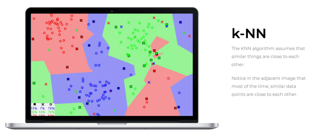
k-NN is recognized as one of the most intuitive and simple classification algorithms in machine learning. Unlike other methods that “learn” patterns in a dataset, k-NN operates on the premise that similar data tend to cluster together in the feature space. This means that k-NN uses the distance between feature vectors to make its predictions, directly depending on this metric to classify new points.

Consider pairs $(X_1, Y_1), (X_2, Y_2), \dots, (X_n, Y_n)$ in $\mathbb{R}^d \times \{1, 2\}$ , where $X$ represents the attributes of data points in a d-dimensional space, and $Y$ is the label of the class of $X$ , indicating to which of the two classes the point belongs.

Each $X$ conditional on $Y=r$ follows a probability distribution $P_r$ for $r=1, 2$ . This means that, given a specific class label, the distribution of data points in $X$ follows a specific pattern, described by the distribution $P_r$ .

Given a norm $\|\cdot\|$ in $\mathbb{R}^d$ and a point $x \in \mathbb{R}^d$ , we order the training data such that $(X_{(1)}, Y_{(1)}), \dots, (X_{(n)}, Y_{(n)})$ in a way that $\|X_{(1)} - x\| \leq \dots \leq \|X_{(n)} - x\|$ .

In other words, we rearrange the training data based on the proximity of each point $X_i$ to the query point $x$ , from the nearest to the farthest.

Intuition Behind k-NN

Imagine you want to classify the ingredients in your pantry based on two features that you assume can be measured by your discerning taste: sweetness and crunchiness.

Each ingredient has been carefully tasted and measured on an arbitrary scale, and the result can be observed in the image below, taken from the book Machine Learning with R (Brett Lantz, 2019).

Intuition behing k-Nearest Neighbors (k-NN) — Intuition behind k-Nearest Neighbors (k-NN). Source: Machine Learning with R (Brett Lantz, 2019).

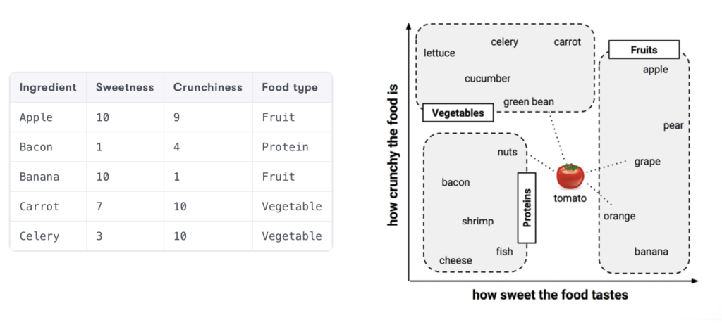
Fruits, generally sweeter, cluster further from the origin along the x-axis, while vegetables, less sweet and more crunchy, and proteins, less sweet and less crunchy, group in distinct areas of the graph. This visual pattern provides a clear clue: sweetness and crunchiness are good indicators for classifying an ingredient from our list.

Now, suppose we have an unknown fruit and want to classify it using k-NN. We start by locating the fruit on the graph based on its sweetness and crunchiness. Then, we select a number $k$ of the closest data points – in this case, the ingredients closest on the graph.

If we choose, for example, $k=3$ , we’ll identify the three ingredients closest to our unknown fruit on the graph. If two of them are ‘fruits’ and one is ‘vegetable’, then, by the majority rule, k-NN will classify the unknown fruit as ‘fruit’. This process is intuitive and mirrors how we often make choices based on obvious similarities.

Obviously, this was a didactic and intuitive example. But to deal with real problems, it’s essential to choose an appropriate value for $k$ and a distance metric that reflects the nature and dimensionality of the data.

Distance Metrics

Distance metrics are fundamental in the k-NN algorithm, as they define how the “closeness” between data points is calculated. Here are some of the most commonly used metrics:

Euclidean Distance: The most common and intuitive among the metrics, used to measure the linear distance between two points, particularly useful when images or data points are represented in Euclidean space, providing a direct measure of the “straight line” between them. If we have two points, $P = (p_1, p_2, ..., p_n)$ and $Q = (q_1, q_2, ..., q_n)$ in an $n$ -dimensional space, the Euclidean distance between them is given by:

$d(P, Q) = \sqrt{(p_1 - q_1)^2 + (p_2 - q_2)^2 + \cdots + (p_n - q_n)^2}$

Manhattan Distance (city block): Also known as L1 norm, this metric measures the distance between two points by moving only in straight lines along the axes (like a taxi moving through a city’s grid of streets), suitable for when the path between points is a grid. For the same points $P$ and $Q$ above, the Manhattan distance is calculated as:

$d(P, Q) = |p_1 - q_1| + |p_2 - q_2| + \cdots + |p_n - q_n|$

Other Metrics: Depending on the type of data and the problem, other distance metrics may be more appropriate, like Minkowski distance. A generalization of Euclidean and Manhattan distances, it’s defined as $(\sum{|p_i - q_i|^r})^{1/r}$ , where $r$ is a parameter that determines the nature of the distance.

How to Choose ‘k’

The choice of $k$ in the k-NN algorithm can vary significantly depending on the dataset. There isn’t a one-size-fits-all rule, but based on experience, here are some general guidelines:

A small $k$ , such as 3 or 5, is often a good choice to avoid the influence of outliers and keep the decision localized close to the query point. However, a very low value can be sensitive to noise in the data.
A larger $k$ offers a more “democratic” decision, considering more neighbors, which can be useful for datasets with a lot of variations. However, a very large value might overly smooth the decision boundaries, leading to less accurate classifications.

A common technique is to use cross-validation to experiment with different $k$ values and choose the one that offers the best performance on the validation set. This helps to find a balance between underfitting and overfitting. Above all, the choice should take into account the insights generated during the business understanding phase.

Classification with K-Nearest Neighbors (k-NN) using Scikit-Learn

Now that we’ve gone through the introduction and conceptualization of k-NN, let’s see how we can use scikit-learn for classification problems in supervised learning. Before moving to a more practical project, let’s first use Python’s numpy library to generate random values and see how they are distributed.

# Importing the necessary libraries

import numpy as np

from sklearn.neighbors import KNeighborsClassifier

import matplotlib.pyplot as plt

# Generating a random dataset

np.random.seed(0)

X = np.random.rand(100, 2) # 100 points in 2 dimensions

y = np.where(X[:, 0] + X[:, 1] > 1, 1, 0) # Classification based on the sum of features

# Visualizing the data

plt.figure(figsize=(8, 6))

plt.scatter(X[y == 0][:, 0], X[y == 0][:, 1], color='red', label='Class 0')

plt.scatter(X[y == 1][:, 0], X[y == 1][:, 1], color='blue', label='Class 1')

plt.title('Generated Dataset')

plt.xlabel('Feature 1')

plt.ylabel('Feature 2')

plt.legend()

plt.show()

# Importing the necessary libraries import numpy as np from sklearn.neighbors import KNeighborsClassifier import matplotlib.pyplot as plt # Generating a random dataset np.random.seed(0) X = np.random.rand(100, 2) # 100 points in 2 dimensions y = np.where(X[:, 0] + X[:, 1] > 1, 1, 0) # Classification based on the sum of features # Visualizing the data plt.figure(figsize=(8, 6)) plt.scatter(X[y == 0][:, 0], X[y == 0][:, 1], color='red', label='Class 0') plt.scatter(X[y == 1][:, 0], X[y == 1][:, 1], color='blue', label='Class 1') plt.title('Generated Dataset') plt.xlabel('Feature 1') plt.ylabel('Feature 2') plt.legend() plt.show()

# Importing the necessary libraries
import numpy as np
from sklearn.neighbors import KNeighborsClassifier
import matplotlib.pyplot as plt

# Generating a random dataset
np.random.seed(0)
X = np.random.rand(100, 2)  # 100 points in 2 dimensions
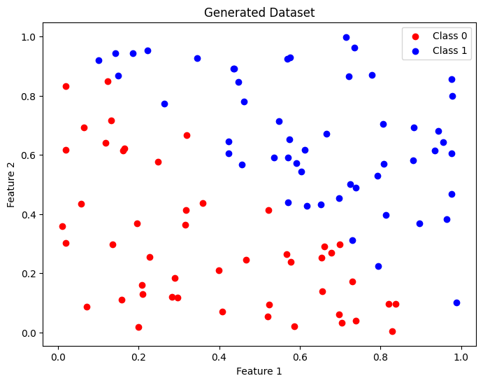
y = np.where(X[:, 0] + X[:, 1] > 1, 1, 0)  # Classification based on the sum of features

# Visualizing the data
plt.figure(figsize=(8, 6))
plt.scatter(X[y == 0][:, 0], X[y == 0][:, 1], color='red', label='Class 0')
plt.scatter(X[y == 1][:, 0], X[y == 1][:, 1], color='blue', label='Class 1')
plt.title('Generated Dataset')
plt.xlabel('Feature 1')
plt.ylabel('Feature 2')
plt.legend()
plt.show()

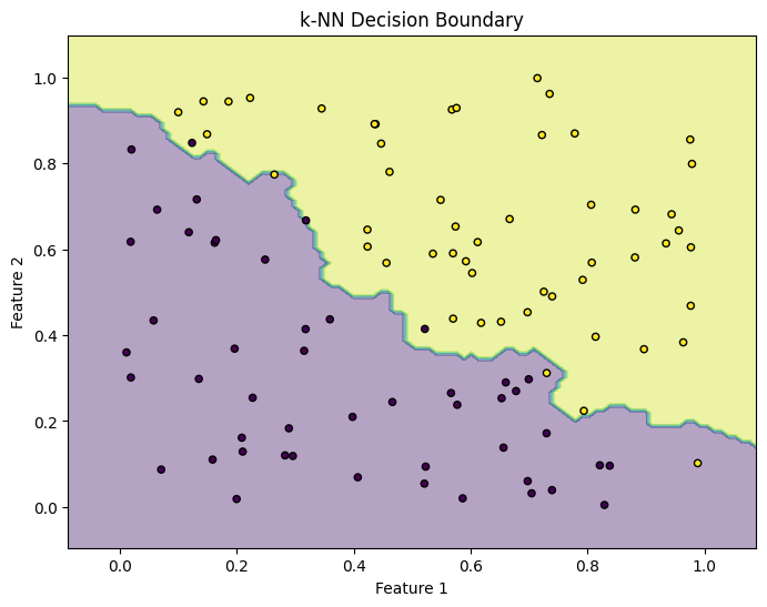
The generated samples were distributed among the labels Class 0 and Class 1. Now, if we want to identify the decision boundary, we first need to train the model. For this, I set the number of nearest neighbors as $k = 3$ , and after instantiating a KNeighborsClassifier object, it’s simply a matter of executing the knn.fit(X, y) method with the synthetic data.

It’s important to remember that during this process, the k-NN model does not learn a discriminative function as in other supervised learning methods; instead, it memorizes the training examples.

Subsequently, when making predictions, it uses these memorized data to find the $k$ nearest neighbors of a new point and carries out a vote based on the labels of these neighbors to determine the classification.

# Defining the number of neighbors

k = 3

# Creating the k-NN model

knn = KNeighborsClassifier(n_neighbors=k)

# Training the model with the generated data

knn.fit(X, y)

# Generating test points for decision boundary visualization

x_min, x_max = X[:, 0].min() - 0.1, X[:, 0].max() + 0.1

y_min, y_max = X[:, 1].min() - 0.1, X[:, 1].max() + 0.1

xx, yy = np.meshgrid(np.linspace(x_min, x_max, 100), np.linspace(y_min, y_max, 100))

Z = knn.predict(np.c_[xx.ravel(), yy.ravel()])

Z = Z.reshape(xx.shape)

# Visualizing the decision boundary

plt.figure(figsize=(8, 6))

plt.contourf(xx, yy, Z, alpha=0.4)

plt.scatter(X[:, 0], X[:, 1], c=y, s=20, edgecolor='k')

plt.title('k-NN Decision Boundary')

plt.xlabel('Feature 1')

plt.ylabel('Feature 2')

plt.show()

# Defining the number of neighbors k = 3 # Creating the k-NN model knn = KNeighborsClassifier(n_neighbors=k) # Training the model with the generated data knn.fit(X, y) # Generating test points for decision boundary visualization x_min, x_max = X[:, 0].min() - 0.1, X[:, 0].max() + 0.1 y_min, y_max = X[:, 1].min() - 0.1, X[:, 1].max() + 0.1 xx, yy = np.meshgrid(np.linspace(x_min, x_max, 100), np.linspace(y_min, y_max, 100)) Z = knn.predict(np.c_[xx.ravel(), yy.ravel()]) Z = Z.reshape(xx.shape) # Visualizing the decision boundary plt.figure(figsize=(8, 6)) plt.contourf(xx, yy, Z, alpha=0.4) plt.scatter(X[:, 0], X[:, 1], c=y, s=20, edgecolor='k') plt.title('k-NN Decision Boundary') plt.xlabel('Feature 1') plt.ylabel('Feature 2') plt.show()

# Defining the number of neighbors
k = 3

# Creating the k-NN model
knn = KNeighborsClassifier(n_neighbors=k)

# Training the model with the generated data
knn.fit(X, y)

# Generating test points for decision boundary visualization
x_min, x_max = X[:, 0].min() - 0.1, X[:, 0].max() + 0.1
y_min, y_max = X[:, 1].min() - 0.1, X[:, 1].max() + 0.1
xx, yy = np.meshgrid(np.linspace(x_min, x_max, 100), np.linspace(y_min, y_max, 100))
Z = knn.predict(np.c_[xx.ravel(), yy.ravel()])
Z = Z.reshape(xx.shape)

# Visualizing the decision boundary
plt.figure(figsize=(8, 6))
plt.contourf(xx, yy, Z, alpha=0.4)
plt.scatter(X[:, 0], X[:, 1], c=y, s=20, edgecolor='k')
plt.title('k-NN Decision Boundary')
plt.xlabel('Feature 1')
plt.ylabel('Feature 2')
plt.show()

In this basic example, the aim was merely to demonstrate the implementation and application of k-NN on a synthetic dataset. But why not take advantage of the momentum and use the same technique to classify RR Lyrae stars?

Applying k-NN to Classify RR Lyrae Stars

In this final part of the article, we will use the k-NN algorithm to classify RR Lyrae variable stars, a distinct type of pulsating stars used as important astronomical markers to measure the galaxy and the expansion of the universe.

SDSS Photometric Filters and Stellar Spectrum, where each colored curve represents one filter (u, g, r, i, z). **Source:** Ivezić et al. (2019).

RR Lyrae stars have well-defined periodic characteristics, which allow astronomers to identify them and study their properties in detail. The dataset we will use can be easily downloaded through the astroML package.

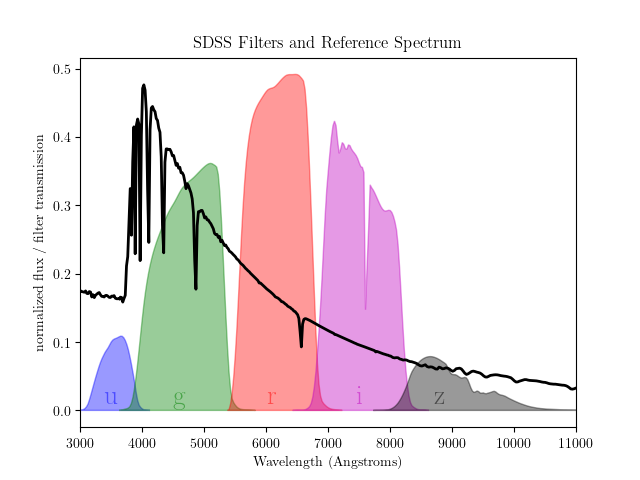
Specifically, the function fetch_rrlyrae_combined does the job of combining photometric data of RR Lyrae stars with standard colors from the Sloan Digital Sky Survey (SDSS), returning the difference between the magnitudes measured in each of the five photometric filters:

X: The feature matrix, containing the color differences (u-g, g-r, r-i, i-z) between the 5 filters for each star. Thus, the dimensionality of X is $(n\_samples, 4)$ , where each column represents one of the calculated color differences.
y: The label vector, where 1 indicates an RR Lyrae star and 0 a background star.

# Importing the necessary libraries

from sklearn.model_selection import train_test_split

from sklearn.neighbors import KNeighborsClassifier

from sklearn.metrics import classification_report, confusion_matrix, accuracy_score

from astroML.datasets import fetch_rrlyrae_combined

import numpy as np # Adding this import for array operations

# Defining the directory where the data will be saved

DATA_HOME = './data'

# Loading the data

X, y = fetch_rrlyrae_combined(data_home=DATA_HOME)

# Initial exploration

print("Shape of X:", X.shape)

print("Shape of y:", y.shape)

print("Number of RR Lyrae stars:", np.sum(y == 1))

print("Number of background stars:", np.sum(y == 0))

# Statistical analysis

print("Basic statistics for each column of X (u-g, g-r, r-i, i-z):")

print("Mean:", np.mean(X, axis=0))

print("Median:", np.median(X, axis=0))

print("Standard deviation:", np.std(X, axis=0))

# Importing the necessary libraries from sklearn.model_selection import train_test_split from sklearn.neighbors import KNeighborsClassifier from sklearn.metrics import classification_report, confusion_matrix, accuracy_score from astroML.datasets import fetch_rrlyrae_combined import numpy as np # Adding this import for array operations # Defining the directory where the data will be saved DATA_HOME = './data' # Loading the data X, y = fetch_rrlyrae_combined(data_home=DATA_HOME) # Initial exploration print("Shape of X:", X.shape) print("Shape of y:", y.shape) print("Number of RR Lyrae stars:", np.sum(y == 1)) print("Number of background stars:", np.sum(y == 0)) # Statistical analysis print("Basic statistics for each column of X (u-g, g-r, r-i, i-z):") print("Mean:", np.mean(X, axis=0)) print("Median:", np.median(X, axis=0)) print("Standard deviation:", np.std(X, axis=0))

# Importing the necessary libraries
from sklearn.model_selection import train_test_split
from sklearn.neighbors import KNeighborsClassifier
from sklearn.metrics import classification_report, confusion_matrix, accuracy_score
from astroML.datasets import fetch_rrlyrae_combined
import numpy as np  # Adding this import for array operations

# Defining the directory where the data will be saved
DATA_HOME = './data'

# Loading the data
X, y = fetch_rrlyrae_combined(data_home=DATA_HOME)

# Initial exploration
print("Shape of X:", X.shape)
print("Shape of y:", y.shape)
print("Number of RR Lyrae stars:", np.sum(y == 1))
print("Number of background stars:", np.sum(y == 0))

# Statistical analysis
print("Basic statistics for each column of X (u-g, g-r, r-i, i-z):")
print("Mean:", np.mean(X, axis=0))
print("Median:", np.median(X, axis=0))
print("Standard deviation:", np.std(X, axis=0))

Shape of X: (93141, 4)
Shape of y: (93141,)
Number of RR Lyrae stars: 483
Number of background stars: 92658
Basic statistics for each column of X (u-g, g-r, r-i, i-z):
Mean: [0.9451376 0.3240073 0.12292135 0.0672943 ]
Median: [0.941 0.33600044 0.12800026 0.05599976]
Standard deviation: [0.10446888 0.06746367 0.04031635 0.05786987]

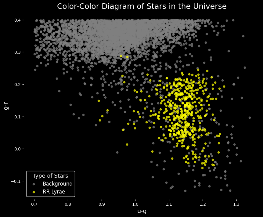
After executing the above cell, the data will be downloaded into the ./data folder. Let’s take this opportunity to quickly look at a sample of the dataset and make a visual comparison between the two classes.

# Selecting a sample for easier visualization

X_sample = X[-5000:]

y_sample = y[-5000:]

# Split stars from RR Lyrae based on the value of y

X_rrlyrae = X_sample[y_sample == 1]

X_background = X_sample[y_sample == 0]

# Creating an enhanced scatter plot of the data with a black background

plt.style.use('dark_background')

fig, ax = plt.subplots(figsize=(10, 8))

# Plotting background stars

ax.scatter(X_background[:, 0], X_background[:, 1], color='grey', s=20, label='Background', alpha=0.7)

# Plotting RR Lyrae stars

ax.scatter(X_rrlyrae[:, 0], X_rrlyrae[:, 1], color='yellow', s=20, label='RR Lyrae', alpha=0.7)

# Enhancing the plot with titles and labels

ax.set_title('Color-Color Diagram of Stars in the Universe', fontsize=18, color='white')

ax.set_xlabel('u-g', fontsize=14, color='white')

ax.set_ylabel('g-r', fontsize=14, color='white')

# Remove grid and borders

ax.grid(False)

for spine in ax.spines.values():

spine.set_visible(False)

# Adding a legend with a white font color

ax.legend(title='Type of Stars', title_fontsize='13', fontsize='12', facecolor='black', edgecolor='white', labelcolor='white')

# Displaying the plot

plt.show()

# Selecting a sample for easier visualization X_sample = X[-5000:] y_sample = y[-5000:] # Split stars from RR Lyrae based on the value of y X_rrlyrae = X_sample[y_sample == 1] X_background = X_sample[y_sample == 0] # Creating an enhanced scatter plot of the data with a black background plt.style.use('dark_background') fig, ax = plt.subplots(figsize=(10, 8)) # Plotting background stars ax.scatter(X_background[:, 0], X_background[:, 1], color='grey', s=20, label='Background', alpha=0.7) # Plotting RR Lyrae stars ax.scatter(X_rrlyrae[:, 0], X_rrlyrae[:, 1], color='yellow', s=20, label='RR Lyrae', alpha=0.7) # Enhancing the plot with titles and labels ax.set_title('Color-Color Diagram of Stars in the Universe', fontsize=18, color='white') ax.set_xlabel('u-g', fontsize=14, color='white') ax.set_ylabel('g-r', fontsize=14, color='white') # Remove grid and borders ax.grid(False) for spine in ax.spines.values(): spine.set_visible(False) # Adding a legend with a white font color ax.legend(title='Type of Stars', title_fontsize='13', fontsize='12', facecolor='black', edgecolor='white', labelcolor='white') # Displaying the plot plt.show()

# Selecting a sample for easier visualization
X_sample = X[-5000:]
y_sample = y[-5000:]

# Split stars from RR Lyrae based on the value of y
X_rrlyrae = X_sample[y_sample == 1]
X_background = X_sample[y_sample == 0]

# Creating an enhanced scatter plot of the data with a black background
plt.style.use('dark_background')
fig, ax = plt.subplots(figsize=(10, 8))

# Plotting background stars
ax.scatter(X_background[:, 0], X_background[:, 1], color='grey', s=20, label='Background', alpha=0.7)

# Plotting RR Lyrae stars
ax.scatter(X_rrlyrae[:, 0], X_rrlyrae[:, 1], color='yellow', s=20, label='RR Lyrae', alpha=0.7)

# Enhancing the plot with titles and labels
ax.set_title('Color-Color Diagram of Stars in the Universe', fontsize=18, color='white')
ax.set_xlabel('u-g', fontsize=14, color='white')
ax.set_ylabel('g-r', fontsize=14, color='white')

# Remove grid and borders
ax.grid(False)
for spine in ax.spines.values():
    spine.set_visible(False)

# Adding a legend with a white font color
ax.legend(title='Type of Stars', title_fontsize='13', fontsize='12', facecolor='black', edgecolor='white', labelcolor='white')

# Displaying the plot
plt.show()

The first step in the code is to split the data into training and test sets using the train_test_split function from the sklearn.model_selection module. The test_size parameter is set to 0.2, meaning that 20% of the data will be used for testing and the remaining 80% for training. The random_state parameter is set to 42 to ensure that the splits generated are reproducible.

Next, the KNN classifier is initialized with n_neighbors=5, given that the number of entries is considerably larger than in our first example from the article. The classifier is then trained using the fit method, which takes the training data and labels as arguments.

Once the training phase is completed, the classifier can be tested using the predict() method. As you can follow, the test data were used to evaluate the classifier’s performance, along with the classification_report, confusion_matrix, and accuracy_score functions. Finally, I included two plots for a visual comparison.

# Splitting the data into training and test sets

X_train, X_test, y_train, y_test = train_test_split(X, y, test_size=0.2, random_state=42)

# Train the classifier

knn = KNeighborsClassifier(n_neighbors=5)

knn.fit(X_train, y_train)

# Test the classifier

y_pred = knn.predict(X_test)

# Evaluate the classifier

print("Classification Report:\n", classification_report(y_test, y_pred))

print("Confusion Matrix:\n", confusion_matrix(y_test, y_pred))

print("Accuracy:", accuracy_score(y_test, y_pred))

# Plot the results

plt.figure(figsize=(12, 6))

plt.subplot(1, 2, 1)

plt.scatter(X_test[y_test == 0][:, 0], X_test[y_test == 0][:, 1], color='red', label='Background', s=10)

plt.scatter(X_test[y_test == 1][:, 0], X_test[y_test == 1][:, 1], color='blue', label='RR Lyrae', s=10)

plt.title('Real Test Data')

plt.xlabel('u-g')

plt.ylabel('g-r')

plt.legend()

plt.subplot(1, 2, 2)

plt.scatter(X_test[y_pred == 0][:, 0], X_test[y_pred == 0][:, 1], color='red', label='Background', s=10)

plt.scatter(X_test[y_pred == 1][:, 0], X_test[y_pred == 1][:, 1], color='blue', label='RR Lyrae', s=10)

plt.title('Predicted Test Data')

plt.xlabel('u-g')

plt.ylabel('g-r')

plt.legend()

plt.show()

# Splitting the data into training and test sets X_train, X_test, y_train, y_test = train_test_split(X, y, test_size=0.2, random_state=42) # Train the classifier knn = KNeighborsClassifier(n_neighbors=5) knn.fit(X_train, y_train) # Test the classifier y_pred = knn.predict(X_test) # Evaluate the classifier print("Classification Report:\n", classification_report(y_test, y_pred)) print("Confusion Matrix:\n", confusion_matrix(y_test, y_pred)) print("Accuracy:", accuracy_score(y_test, y_pred)) # Plot the results plt.figure(figsize=(12, 6)) plt.subplot(1, 2, 1) plt.scatter(X_test[y_test == 0][:, 0], X_test[y_test == 0][:, 1], color='red', label='Background', s=10) plt.scatter(X_test[y_test == 1][:, 0], X_test[y_test == 1][:, 1], color='blue', label='RR Lyrae', s=10) plt.title('Real Test Data') plt.xlabel('u-g') plt.ylabel('g-r') plt.legend() plt.subplot(1, 2, 2) plt.scatter(X_test[y_pred == 0][:, 0], X_test[y_pred == 0][:, 1], color='red', label='Background', s=10) plt.scatter(X_test[y_pred == 1][:, 0], X_test[y_pred == 1][:, 1], color='blue', label='RR Lyrae', s=10) plt.title('Predicted Test Data') plt.xlabel('u-g') plt.ylabel('g-r') plt.legend() plt.show()

# Splitting the data into training and test sets
X_train, X_test, y_train, y_test = train_test_split(X, y, test_size=0.2, random_state=42)

# Train the classifier
knn = KNeighborsClassifier(n_neighbors=5)
knn.fit(X_train, y_train)

# Test the classifier
y_pred = knn.predict(X_test)

# Evaluate the classifier
print("Classification Report:\n", classification_report(y_test, y_pred))
print("Confusion Matrix:\n", confusion_matrix(y_test, y_pred))
print("Accuracy:", accuracy_score(y_test, y_pred))

# Plot the results
plt.figure(figsize=(12, 6))
plt.subplot(1, 2, 1)
plt.scatter(X_test[y_test == 0][:, 0], X_test[y_test == 0][:, 1], color='red', label='Background', s=10)
plt.scatter(X_test[y_test == 1][:, 0], X_test[y_test == 1][:, 1], color='blue', label='RR Lyrae', s=10)
plt.title('Real Test Data')
plt.xlabel('u-g')
plt.ylabel('g-r')
plt.legend()

plt.subplot(1, 2, 2)
plt.scatter(X_test[y_pred == 0][:, 0], X_test[y_pred == 0][:, 1], color='red', label='Background', s=10)
plt.scatter(X_test[y_pred == 1][:, 0], X_test[y_pred == 1][:, 1], color='blue', label='RR Lyrae', s=10)
plt.title('Predicted Test Data')
plt.xlabel('u-g')
plt.ylabel('g-r')
plt.legend()

plt.show()

Classification Report:

precision recall f1-score support

0.0 1.00 1.00 1.00 18530

1.0 0.67 0.61 0.63 99

accuracy 1.00 18629

macro avg 0.83 0.80 0.82 18629

weighted avg 1.00 1.00 1.00 18629

Confusion Matrix:

[[18500 30]

[ 39 60]]

Accuracy: 0.9962960974824199

Classification Report: precision recall f1-score support 0.0 1.00 1.00 1.00 18530 1.0 0.67 0.61 0.63 99 accuracy 1.00 18629 macro avg 0.83 0.80 0.82 18629 weighted avg 1.00 1.00 1.00 18629 Confusion Matrix: [[18500 30] [ 39 60]] Accuracy: 0.9962960974824199

Classification Report:
               precision    recall  f1-score   support

         0.0       1.00      1.00      1.00     18530
         1.0       0.67      0.61      0.63        99

    accuracy                           1.00     18629
   macro avg       0.83      0.80      0.82     18629
weighted avg       1.00      1.00      1.00     18629

Confusion Matrix:
 [[18500    30]
 [   39    60]]
Accuracy: 0.9962960974824199

The analysis of the presented results reveals satisfactory performance for a simple classification model, like k-NN. The report indicates that the model is highly accurate in identifying Background and is also effective in retrieving instances of this class. On the other hand, RR Lyrae, which is of greater interest to us, shows inferior performance, with a precision of 0.67 and recall of 0.61, indicating that the model is reasonably accurate but is missing some instances of this class.

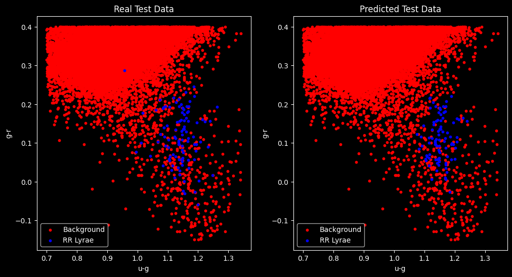
The F1-score metric, which combines precision and recall, is 0.63 for class 1.0. The overall accuracy is 0.996, suggesting that the model is making correct predictions in the vast majority of instances. The confusion matrix also provides detailed information about true positives, false positives, true negatives, and false negatives.

However, for the purposes of this article, the model serves its educational objective, demonstrating how quick and simple k-NN can be as a classification tool.

Conclusion

In this article, you were introduced to the K-Nearest Neighbors (KNN) classification model and learned how to implement it for the task of classifying RR Lyrae stars using the scikit-learn library.

In the real world, the choice of classification algorithm depends on the nature of the data and the objectives of the project. However, what we are currently seeing are professionals who are eager to learn in practice, tools that are fashionable, and sometimes forget to invest time to reinforce their theoretical foundation.

The truth is that KNN is just one of the many tools available to data scientists, and it can be the best choice in various types of situations. After all, just as you would not use an AIM-9X Sidewinder missile to eliminate a cockroach (even a tough one!), wanting to use Deep Learning for all situations can be a symptom that you still don’t know the classic and veteran tools, already validated in real combat.