Histogram Equalization with OpenCV and Python

Histogram is a concept that is present directly or indirectly in practically all computer vision applications. In histogram equalization, we aim for the full spectrum of intensities, distributing the pixel values more evenly along the x-axis.

After all, by adjusting the distribution of pixel values, we can enhance details and reveal characteristics that were previously hidden in the original image.

Therefore, understanding the concept and learning how to apply the technique is fundamental for working on digital image processing problems. In this tutorial, you will learn the theory and how to equalize histograms in digital images using OpenCV and Python.

Click here to download the source code to this post

What is an Image Histogram

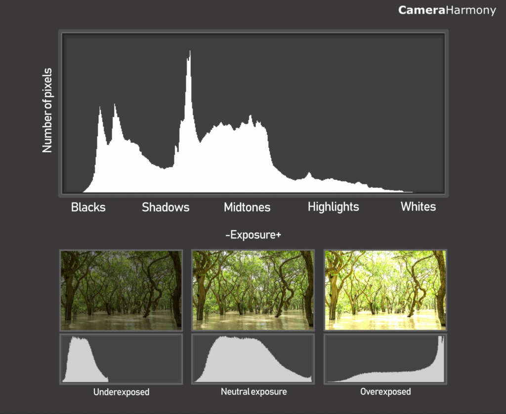
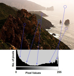
An image histogram is a type of graphical representation that shows how the intensities of the pixels of a given digital image are distributed.

In simple terms, a histogram will tell you if an image is correctly exposed, if the lighting is adequate, and if the contrast allows highlighting some desirable features.

A histogram is a graphical representation of how pixel intensity values are distributed in your image. — A histogram is a graphical representation of how pixel intensity values are distributed in your image (source).

We use histograms to identify spectral signatures in hyperspectral satellite images – such as distinguishing between genetically modified and organic crops.

We use histograms to segment parts on a factory conveyor belt – applying thresholding to isolate objects.

And looking at various algorithms like SIFT and HOG, the use of image gradient histograms is fundamental for the detection and description of robust local features.

Examples of pixels and their intensity values distributed in the histogram (source).

This technique is fundamental in digital image processing and is widely used in various fields, including the medical area, such as in X-ray and CT scans.

Besides being a fundamental tool, as it is very simple to calculate, it is a very popular alternative for applications that require real-time processing.

Formal Definition

A histogram of a digital image $f(x, y)$ whose intensities vary in the range $[0, L - 1]$ is a discrete function

$h(r_{k}) = n_{k},$

where $r_k$ is the $k$ -th intensity value and $n_k$ is the total number of pixels in $f$ with intensity $r_k$ . Similarly, the normalized histogram of a digital image $f(x, y)$ is

$p(r_{k}) = \frac{h(r_{k})}{MN} = \frac{n_k}{MN},$

where $M$ and $N$ are the dimensions of the image (rows and columns, respectively). It is common practice to divide each component of a histogram by the total number of pixels to normalize it.

Since $p(r_k)$ is the probability of occurrence of a given intensity level $r_k$ in an image, the sum of all components equals $1$ .

How to Calculate a Histogram

Manually calculating an image histogram is a straightforward process that involves counting the frequency of each pixel intensity value in an image.

For educational purposes, I have provided pseudocode and an implementation using numpy to demonstrate how to do this.

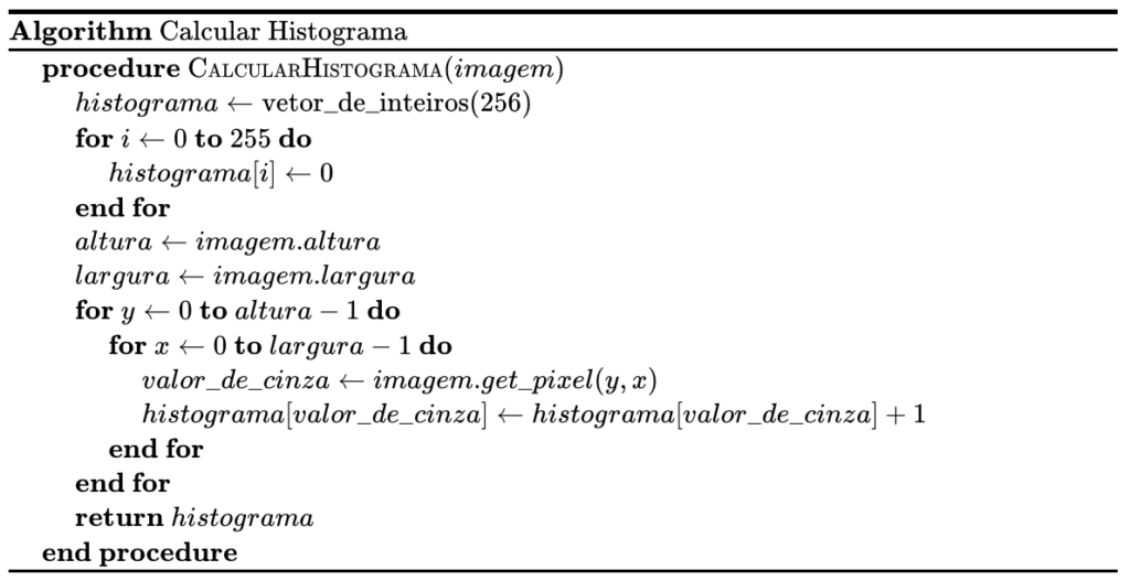
First, we initialize a vector to store the histogram with zeros. In this case, I am considering an 8-bit grayscale image ( $2^8 = 256$ ) possible values for each pixel intensity.

Next, we capture the image’s height and width attributes. If necessary, we could also include the channels attribute.

Then, we iterate over each pixel of the image, incrementing the corresponding position in the histogram vector based on the pixel intensity value. This way, at the end of the process, the histogram vector will contain the count of occurrences of each gray level in the image, providing a clear representation of the intensity distribution in the image.

Histogram Calculation in NumPy

The NumPy library has the np.histogram() function, which allows calculating histograms of input data. This function is quite flexible and can handle different bin configurations and ranges.

numpy.histogram(
    a: np.ndarray,
    bins: Union[int, np.ndarray, str] = 10,
    range: Optional[Tuple[float, float]] = None,
    density: Optional[bool] = None,
    weights: Optional[np.ndarray] = None
) -> Tuple[np.ndarray, np.ndarray]

See the example usage in the code below and note that when we use np.histogram() to calculate the histogram of a grayscale image, we set the number of bins to 256 to cover all pixel intensity values from 0 to 255.

However, it’s essential to understand how the library calculates the bins. NumPy calculates them in intervals such as $0-0.99$ , $1-1.99$ , up to $255-255.99$ . Practically, this means there will be 257 elements in the bins array (since we passed the argument $256$ in the function).

As we don’t need this extra value, as pixel intensity values range between $0-255$ , we can ignore it.

import cv2
import numpy as np
import matplotlib.pyplot as plt

# Load an image in grayscale
image_path = "carlos_hist.jpg"
image = cv2.imread(image_path, 0)

# Calculate the histogram
hist, bins = np.histogram(image.flatten(), 256, [0, 256])

# Compute the cumulative distribution function
cdf = hist.cumsum()
cdf_normalized = cdf * hist.max() / cdf.max()

Initially, we load the image carlos_hist.jpg in grayscale using the flag $0$ in cv2.imread(image_path, 0). With the image loaded, our next step is to calculate the histogram. We use the np.histogram() function from NumPy for this. This function counts the frequency of occurrence of each pixel intensity value.

To better understand the intensity distribution, we will also calculate the cumulative distribution function (CDF). The CDF is essential for techniques like histogram equalization.

# Plot histogram and C.D.F.
fig, axs = plt.subplots(1, 2, figsize=(10, 5))

# Show the image in grayscale
axs[0].imshow(image, cmap="gray", vmin=0, vmax=255)
axs[0].axis("off")

# Plot the histogram and the CDF
axs[1].plot(cdf_normalized, color="black", linestyle="--", linewidth=1)
axs[1].hist(image.flatten(), 256, [0, 256], color="r", alpha=0.5)
axs[1].set_xlim([0, 256])
axs[1].legend(("CDF", "Histogram"), loc="upper left")

plt.show()

Now, let’s visualize the histogram and the CDF side by side using Matplotlib and setting up our figure with subplots.

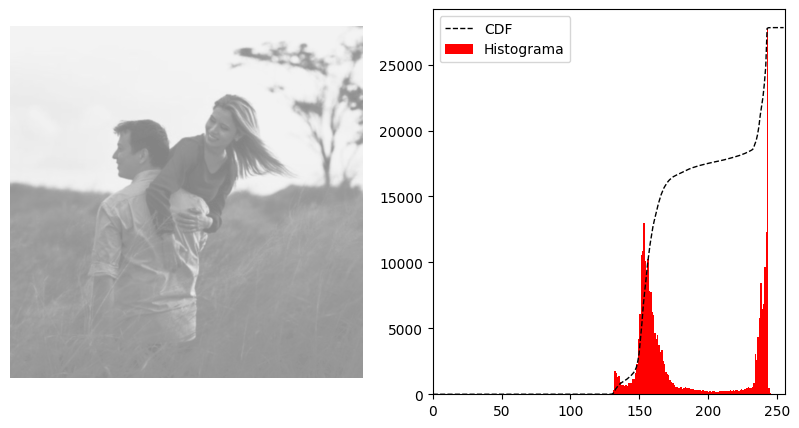Visually, just by looking at the image, we can see that it looks “flat“, with little contrast. This is indeed corroborated by the histogram on the right.

As most pixel intensity values are concentrated around 150, the image has a predominance of mid to light tones, resulting in a less vibrant appearance with little contrast variation.

Histogram Equalization for Grayscale Images

As we mentioned at the beginning of the article, histogram equalization is a technique to adjust the contrast of an image by distributing pixel values more uniformly across the intensity range.

There are several possible techniques, depending on the context, number of channels, and application. In this section, I will show you how to use the cv.equalizeHist() function to perform this process on grayscale images.

cv2.equalizeHist(
    src: np.ndarray
) -> np.ndarray:

The cv2.equalizeHist function equalizes the histogram of the input image using the following algorithm:

Calculate the histogram $( H )$ for src.
Normalize the histogram so that the sum of the histogram bins is 255.
Calculate the cumulative histogram:
$H'_i = \sum_{0 \leq j < i} H(j)$
Transform the image using ( H’ ) as a look-up table:
$\text{dst}(x,y) = H'(\text{src}(x,y))$

To see how this function normalizes the brightness and increases the contrast of the original image, let’s run the code below.

# Apply histogram equalization
equalized = cv2.equalizeHist(image)

# Create a figure with subplots to compare the images
plt.figure(figsize=(30, 10))

# Show equalized image
plt.subplot(1, 3, 1)
plt.imshow(equalized, cmap='gray', vmin=0, vmax=255)
plt.title('Equalized Image')

# Compare original and equalized histograms
plt.subplot(1, 3, 2)
plt.hist(image.flatten(), 256, [0, 256])
plt.title('Original Histogram')
plt.subplot(1, 3, 3)
plt.hist(equalized.flatten(), 256, [0, 256])
plt.title('Equalized Histogram')
plt.show()

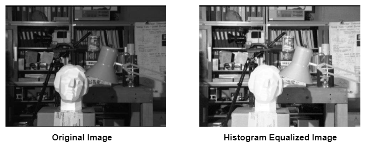
First, we apply histogram equalization to the loaded image using the cv2.equalizeHist function. Next, we create a figure with subplots to analyze the final result.

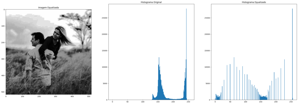The first subplot shows the equalized image, while the next two subplots compare the histograms of the original and processed images, using plt.hist to plot them directly. Notice how the distribution change made the image more visually appealing.

Histogram Equalization for Color Images

If we try to perform histogram equalization on color images by treating each of the three channels separately, we will get a poor and unexpected result.

The reason is that when each color channel is transformed in a non-linear and independent manner, completely new colors that are not related in any way may be generated.

The correct way to perform histogram equalization on color images involves a prior step, which is conversion to a color space like HSV, where intensity is separated:

Transform the image to the HSV color space.
Perform histogram equalization only on the V (Value) channel.
Transform the image back to the RGB color space.

# Read the astrophoto
astrophoto = cv2.imread('astrophoto.jpg')

# Convert to HSV color space
hsv_astrophoto = cv2.cvtColor(astrophoto, cv2.COLOR_BGR2HSV)

# Split the HSV channels
h, s, v = cv2.split(hsv_astrophoto)

First, we load a new color image using cv2.imread. Then, we convert the originally loaded image in BGR format to the HSV color space with cv2.cvtColor and separate the color information (Hue and Saturation) from the intensity (Value) using cv2.split(hsv_astrophoto).

# Equalize the V (Value) channel
v_equalized = cv2.equalizeHist(v)

# Merge the HSV channels back, with the equalized V channel
hsv_astrophoto = cv2.merge([h, s, v_equalized])

# Convert back to RGB color space
astrophoto_equalized = cv2.cvtColor(hsv_astrophoto, cv2.COLOR_HSV2RGB)

After applying histogram equalization only to the V channel, we merge the HSV channels back but replace the V channel with the equalized channel.

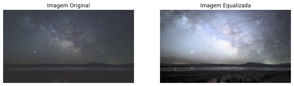
The redistribution of intensity values in the V channel significantly improved the contrast of the image, highlighting details that may have been obscured.

However, the histogram equalization we just saw may not be the best approach in many cases, as it considers the global contrast of the image. In situations where there are large variations in intensity, with very bright and very dark pixels present, or where we would like to enhance only one region of the image, this method may cause us to lose a lot of information.

To address these issues, let’s look at a more advanced technique called Contrast Limited Adaptive Histogram Equalization (CLAHE).

Contrast Limited Adaptive Histogram Equalization (CLAHE)

Contrast Limited Adaptive Histogram Equalization (CLAHE) is a technique that divides the image into small regions called “tiles” and applies histogram equalization to each of these regions independently.

This allows the contrast to be improved locally, preserving details and reducing noise. Additionally, the CLAHE method has the ability to limit the increase in contrast (hence the term “Contrast Limited”), preventing noise amplification that may occur in the regular technique.

cv2.createCLAHE(
    clipLimit: float = 40.0,
    tileGridSize: Optional[Tuple[int, int]] = (8, 8)
) -> cv2.CLAHE:

The implementation of CLAHE in OpenCV is done using the createCLAHE() function. First, a CLAHE object is created with two optional arguments: clipLimit and tileGridSize.

In this last example, let’s use a photo I took with my wife at the Chapada dos Veadeiros National Park in Brazil.

# Read the chapada image
chapada = cv2.imread('chapada.png')

# Convert to HSV color space
chapada_hsv = chapada.copy()
chapada_hsv = cv2.cvtColor(chapada, cv2.COLOR_BGR2HSV)

# Create a CLAHE object
clahe = cv2.createCLAHE(clipLimit=2.0, tileGridSize=(8, 8))
chapada_hsv[:, :, 2] = clahe.apply(chapada_hsv[:, :, 2])

# Convert back to RGB color space
chapada_equalized = cv2.cvtColor(chapada_hsv, cv2.COLOR_HSV2BGR)

After loading the image chapada.png, we convert it to the HSV color space to maintain consistency. Then, we apply CLAHE to the V channel using the cv2.createCLAHE(clipLimit=2.0, tileGridSize=(8, 8)) function. Finally, we convert the image back to the RGB color space to visualize the result.

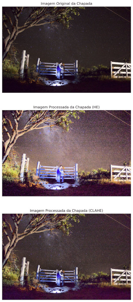
In the original image, there was a well-lit region (fence, tree, and me and my wife). If we had opted for global histogram equalization, the entire image would have been adjusted uniformly, potentially leading to a loss of details in very bright or very dark areas.

However, by using CLAHE, the algorithm used the local context, adapting the number of tiles to adjust the contrast of each small region of the image individually. This preserved details in both bright and dark areas, resulting in a final image with enhanced contrast and more natural colors.

Takeaways

Image Histogram: An image histogram graphically represents the distribution of pixel intensities, indicating whether an image is correctly exposed and helping to enhance hidden details.
Histogram Usage: Histograms are used for various applications, including the segmentation of parts on factory conveyors, identifying spectral signatures in hyperspectral images, and detecting robust local features with algorithms like SIFT and HOG.
Formal Definition: The histogram of a digital image is a discrete function that counts the frequency of each pixel intensity value, which can be normalized to represent the probability of occurrence of each intensity level.
Histogram Equalization for Grayscale Images: The cv2.equalizeHist() function in OpenCV adjusts the contrast of a grayscale image by distributing pixel values more uniformly across the intensity range.
Limitations of Global Equalization: Global histogram equalization may not be ideal in cases with large intensity variations, as it can lead to information loss in very bright or dark areas of the image.
Histogram Equalization for Color Images: When handling color images, histogram equalization should be applied to the intensity (V) channel of the HSV color space to avoid generating unnatural colors.
CLAHE – Contrast Limited Adaptive Histogram Equalization: CLAHE divides the image into small regions and applies histogram equalization locally, preserving details and avoiding noise amplification. This technique is effective for improving the contrast of images with large variations in lighting.

Cite this Post

Use the entry below to cite this post in your research:

Carlos Melo. “Histogram Equalization with OpenCV and Python”, Sigmoidal.AI, 2024, https://sigmoidal.ai/en/histogram-equalization-with-opencv-and-python/.

@incollection{CMelo_HistogramEqualization,
    author = {Carlos Melo},
    title = {Histogram Equalization with OpenCV and Python},
    booktitle = {Sigmoidal.ai},
    year = {2024},
    url = {https://sigmoidal.ai/en/histogram-equalization-with-opencv-and-python/},
}