Grad-CAM: Visualizing What a Neural Network Sees

You’ve trained a neural network, but have no idea what it’s actually looking at to make its decisions? The truth is that deep neural networks, especially deep learning models, work as black boxes. You feed in an image, get a prediction, but what happens between input and output remains a mystery.

Grad-CAM (Gradient-weighted Class Activation Mapping) solves exactly that. It generates a heatmap showing which regions of the image were most important for the model’s decision. It’s like asking the neural network to grab a highlighter and mark what it looked at before answering.

In this article, we’ll implement Grad-CAM from scratch with PyTorch, apply it to a ResNet18 trained to classify 102 flower species, and visually analyze what changes when the model gets it right versus when it gets it wrong.

💡 Notebook: Grad-CAM Visualizing CNNs

What Is Grad-CAM?

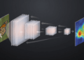
Convolutional networks learn hierarchical filters: the early layers detect edges and textures, the middle layers combine these patterns into object parts, and the final layers recognize whole objects. If you want to know what your network has learned, the right place to look is the last convolutional layer, where the filters carry the richest and most abstract information about the image.

Grad-CAM, proposed by Selvaraju et al. (ICCV 2017), does exactly that. It uses the gradients flowing into the last convolutional layer to compute the importance of each activation channel. Channels that strongly influence a class prediction receive high weight. Irrelevant channels receive low weight. The result is a heatmap highlighting the image regions that contributed most to the decision.

Think of it this way: when you ask “why do you think this is a rose?”, Grad-CAM is the network’s visual answer. It points to the petals, the flower’s shape, the features that led to that class.

How It Works: From Gradients to Heatmap

The Grad-CAM algorithm has four steps:

1. Forward pass: the image passes through the network normally. We capture the activations from the last convolutional layer (a tensor with multiple channels, each highlighting different patterns).

1. Backward pass: we run backpropagation from the predicted class. We capture the gradients arriving at that same layer.

1. Per-channel weights: for each channel, we compute the global average of the gradients (Global Average Pooling). This gives us a scalar weight per channel, representing “how much this channel matters for the predicted class.”

1. Weighted combination: we multiply each activation map by its weight and sum everything. We apply ReLU to keep only positive contributions. The result is the Grad-CAM heatmap.

In mathematical terms:

   

   

Where is the weight for channel , is that channel’s activation map, and is the score for class . The ReLU ensures only regions with positive influence appear in the map.

Implementation with PyTorch Hooks

The most elegant part of the implementation is that we don’t need to modify the network architecture. PyTorch offers hooks — functions that intercept activations and gradients during the forward and backward pass.

We’ll create a GradCAM class that registers hooks on the output of a ResNet18’s last residual block, layer4[-1]. This position captures activations after batch normalization, skip connection, and ReLU — the standard practice in the literature:

class GradCAM:
    def __init__(self, model, target_layer):
        self.model = model
        self.activations = None
        self.gradients = None

        # Register hooks and save handles for removal
        self._fwd_handle = target_layer.register_forward_hook(self._save_activation)
        self._bwd_handle = target_layer.register_full_backward_hook(self._save_gradient)

    def _save_activation(self, module, input, output):
        self.activations = output.detach()

    def _save_gradient(self, module, grad_input, grad_output):
        self.gradients = grad_output[0].detach()

The two hooks do all the heavy lifting. The forward hook saves the activations as the image passes through the layer. The backward hook saves the gradients during backpropagation. We save the returned handles so we can remove the hooks later, avoiding memory leaks.

Now, the method that generates the heatmap and the method that removes the hooks:

def generate(self, input_img, class_idx=None):
    assert input_img.size(0) == 1, "GradCAM expects batch_size=1"

    self.model.eval()
    output = self.model(input_img)

    if class_idx is None:
        class_idx = output.argmax(dim=1).item()

    self.model.zero_grad()
    output[0, class_idx].backward()

    # Weights: global average of gradients per channel
    weights = self.gradients.mean(dim=[2, 3], keepdim=True)

    # Weighted activation map
    cam = (weights * self.activations).sum(dim=1, keepdim=True)
    cam = torch.relu(cam)

    # Normalize between 0 and 1
    cam = cam - cam.min()
    if cam.max() > 0:
        cam = cam / cam.max()

    return cam.squeeze().cpu().numpy(), class_idx

def remove(self):
    """Remove registered hooks to avoid memory leaks."""
    self._fwd_handle.remove()
    self._bwd_handle.remove()

The weights.mean(dim=[2, 3]) is the Global Average Pooling of the gradients. Each channel gets a scalar weight. The multiplication weights * self.activations weights each activation map by its importance. The sum and ReLU produce the final map. Interpolation to 224×224 is done in the visualization function, keeping the GradCAM class reusable.

Visualizing Where the Network Focuses

We applied Grad-CAM to a ResNet18 fine-tuned with transfer learning on the Oxford Flowers 102 dataset, achieving ~92% validation accuracy and ~90% on the test set. The model learned to distinguish 102 flower species.

For the visualization, we overlay the heatmap on the original image with transparency (alpha = 0.5). Red and yellow regions indicate where the network concentrated its attention. Blue regions were largely ignored.

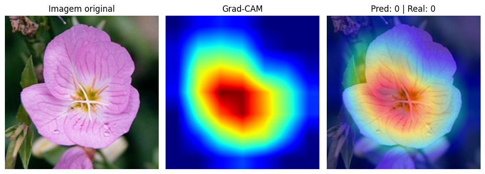
In correct predictions, the pattern is clear: the network focuses on the petals, shape, and central structure of the flower. It learned to ignore leaves, stems, and background, concentrating its attention on the features that truly differentiate one species from another. It’s exactly what a botanist would do when classifying a flower by appearance.

What Changes When the Model Gets It Wrong?

This is where it gets interesting. When we analyze incorrect predictions with Grad-CAM, the heatmap reveals why the model got confused.

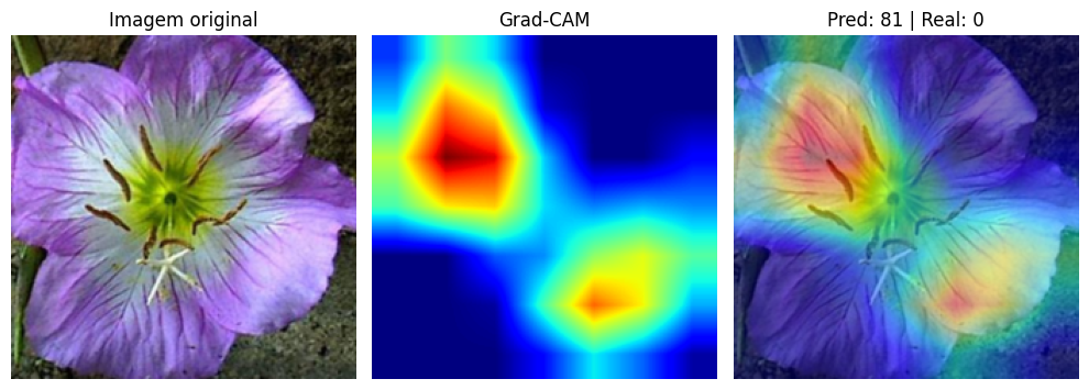
In errors, the network frequently focuses on background regions, edges, or uninformative parts of the image. Instead of looking at the petals, it might pay attention to the stem, the leaves, or even the background texture. The model isn’t necessarily “broken.” It may be using visual shortcuts that worked during training but don’t generalize to that specific image.

This analysis is extremely valuable in practice. If you’re developing a model for production, Grad-CAM lets you diagnose systematic failures. If the model consistently makes mistakes by looking at the background, perhaps the dataset has a bias (red flowers always photographed against a green background, for example). Without Grad-CAM, you’d only see the number of errors, without understanding the cause.

Why Does This Matter?

Explainability is not an academic luxury. In real-world computer vision applications, understanding what the model has learned is just as important as accuracy.

In medicine, a model that classifies tumors by looking at the scale ruler in the image instead of the tissue is dangerous, even if it has high test accuracy. In manufacturing, a visual inspection system that focuses on the conveyor belt background instead of the part can miss defects. Grad-CAM turns the black box into something auditable.

Furthermore, Grad-CAM works with any CNN. If you already have a trained network, just register hooks on the last convolutional layer. No retraining needed, no architecture modifications. A few lines of code to gain an entire layer of interpretability.

Key Takeaways

• Grad-CAM generates heatmaps showing where the CNN looks. It uses gradients from the last convolutional layer to compute the importance of each activation channel, producing a visual map of the most relevant regions for the prediction.

• The PyTorch hooks implementation is simple and non-invasive. Just register a forward hook (activations) and a backward hook (gradients) on the desired layer. No modifications to the network architecture are needed.

• Correct predictions focus on the right features. In correct Oxford Flowers 102 classifications, the network concentrated attention on petals and flower structure, ignoring background and foliage.

• Wrong predictions reveal the reason for the error. When the model gets it wrong, Grad-CAM shows that attention scatters to irrelevant regions. This enables diagnosing systematic failures and dataset bias.

• Explainability is essential for production. A model with 90% accuracy that looks at the wrong place can be more dangerous than one with 85% that looks at the right place. Grad-CAM lets you audit that difference.

Grad-CAM is especially useful in computer vision tasks where confidence in the model needs to be justified.