Building a Deep Learning Neural Network using TensorFlow

In this tutorial, you will learn how to implement Multilayer Neural Networks using Python and the Deep Learning library Keras, one of the most popular libraries currently.

Keras is a Neural Network library that can run with TensorFlow (not only) and was developed to enable easy and fast prototyping. Multilayer Neural Networks are those in which neurons are structured in two or more layers (layers) of processing (since at least there will be 1 input layer and 1 output layer).

.

Implementing a complete Neural Network architecture from scratch is a Herculean task, requiring a more solid understanding of Programming, Linear Algebra, and Statistics – not to mention that the computational performance of your implementation will hardly match the performance of famous libraries in the community.

To show that with a few lines of code, it is possible to implement a simple Network, let’s take the well-known MNIST classification problem and see the performance of our algorithm when submitted to this dataset with 70,000 images!

If you want, all the code will be available on my Github!

Neural Network Architecture

Neural Networks are modeled as a set of neurons connected as an acyclic graph. What does this mean in practice? It means that the outputs of some neurons will be the inputs of other neurons.

The most commonly found Neural Networks out there are those organized into distinct layers (layers), each layer containing a set of neurons. The most commonly found layer type is the fully-connected layer. In this type, neurons between two adjacent layers connect two by two.

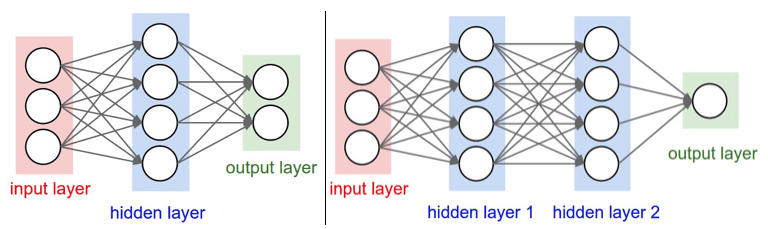
This type of architecture is also known as Feedforward Neural Network because only a neuron from the layer $l_i$ is allowed to connect to a neuron from the layer $l_{I+1}, as illustrated in the figure below.

What is MNIST

MNIST is a dataset containing thousands of handwritten images of digits 0-9. The challenge in this dataset is, given any image, to apply the corresponding label (correctly classify the image). MNIST is so studied and used by the community that it acts as a benchmark to compare different image recognition algorithms.

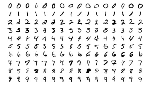
The complete dataset consists of 70,000 images, each 28 x 28 pixels in size. The figure above shows some random examples from the dataset for each of the possible digits. It should be noted that the images are already normalized and centered. Since the images are in grayscale, i.e., they have only one channel, the value corresponding to each pixel in the images should vary within the range [0, 255].

Multilayer Neural Networks are those in which neurons are structured in two or more layers (layers) of processing.
Ian Goodfellow

MNIST in Python

As it is so widely used, the MNIST dataset is already available within the scikit-learn library and can be imported directly by Python with fetch_mldata("MNIST Original"). To illustrate how to import the complete MNIST and extract some basic information, let’s run the code below:

# Importing the necessary libraries
import numpy as np
import matplotlib.pyplot as plt
from keras.datasets import mnist

# Loading the MNIST dataset
(train_images, train_labels), (test_images, test_labels) = mnist.load_data()

# Checking the shape of the data
print("Train Images Shape:", train_images.shape)
print("Train Labels Shape:", train_labels.shape)
print("Test Images Shape:", test_images.shape)
print("Test Labels Shape:", test_labels.shape)

# Visualizing an example image
example_image = train_images[0]
plt.imshow(example_image, cmap='gray')
plt.title(f"Label: {train_labels[0]}")
plt.show()

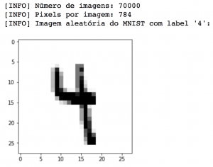
Above, we can see that the array containing the images indeed has 70,000 rows (one row for each image) and 784 columns (all the 28 x 28 pixels of the image). We can also see one of the randomly chosen images. In the case of this digit, our algorithm would have been successful if it could correctly classify the digit as ‘4’.

Implementing our Neural Network with Python and TensorFlow (Keras)

After a brief introduction to Neural Networks, let’s implement a Feedforward Neural Network for the MNIST classification problem. Create a new file in your favorite IDE, named rede_neural_keras.py, and follow the steps of the code below.

# import necessary packages
from sklearn.datasets import fetch_mldata
from sklearn.model_selection import train_test_split
from sklearn.metrics import classification_report
from sklearn.preprocessing import LabelBinarizer
from keras.models import Sequential
from keras.layers.core import Dense
from keras.optimizers import SGD
import numpy as np
import matplotlib.pyplot as plt

Above, we have imported all the necessary packages to create a simple Neural Network with the Keras library. If you encountered an error while trying to import the packages, or do not have a dedicated Python virtual environment for working with Deep Learning/Computer Vision, I recommend looking for a tutorial based on your Operating System.

# import MNIST
print("[INFO] importing MNIST...")
dataset = fetch_mldata("MNIST Original")

# normalize all pixels, so that the values are
# in the range [0, 1.0]
data = dataset.data.astype("float") / 255.0
labels = dataset.target

After importing the set of images, I will divide it into a training set (75%) and a test set (25%), a well-known practice in the Data Science universe. But be careful! The training and test sets MUST BE INDEPENDENT to avoid various problems, including overfitting.

Although it seems complicated, this can be done with just one line of code, thanks to the scikit-learn library, which can be done easily with the train_test_split method. At this stage of preparing our data, we will also need to convert the labels (which are represented by integers) to binary vector format. To illustrate what a binary vector is, see the example below, which indicates the label 4.

4 = [0,0,0,0,1,0,0,0,0,0]

In this vector, the value 1 is assigned to the index corresponding to the label and the value 0 to the others. This operation, known as one-hot encoding, can also be done easily with the LabelBinarizer class.

# split the dataset into train (75%) and test (25%)
(trainX, testX, trainY, testY) = train_test_split(data, dataset.target)

# convert labels from integers to vectors
lb = LabelBinarizer()
trainY = lb.fit_transform(trainY)
testY = lb.transform(testY)

Great! With the dataset imported and processed correctly, we can finally define the architecture of our Neural Network with Keras. Arbitrarily, I defined that the Neural Network will have 4 layers:

1. Our first layer (l0) will receive as input the values ​​related to each pixel of the images. So, since each image has a size equal to 28 x 28 pixels, l0 will have 784 neurons.
2. The hidden layers l1 and l2 will arbitrarily have 128 and 64 neurons.
3. Finally, the last layer, l3, will have the number of neurons corresponding to the number of classes in our classification problem: 10 (remember, there are 10 possible digits).

# define the Neural Network architecture using Keras
# 784 (input) => 128 (hidden) => 64 (hidden) => 10 (output)

model = Sequential()
model.add(Dense(128, input_shape=(784,), activation="sigmoid"))
model.add(Dense(64, activation="sigmoid"))
model.add(Dense(10, activation="softmax"))

Within the concept of feedforward architecture, our Neural Network is instantiated by the Sequential class, which means that each layer will be “stacked” on top of another, with the output of one being the input of the next. In our example, all layers are of the fully-connected layer type.

The hidden layers will be activated by the sigmoid function, which takes the real values of the neurons as input and places them within the range [0, 1]. For the last layer, which needs to reflect the probabilities for each of the possible classes, the softmax function will be used.

To train our model, I will use the most important algorithm for Neural Networks: Stochastic Gradient Descent (SGD). I want to make a dedicated post about SGD in the future (mathematics + code), given its importance! But for now, let’s use the algorithm already available in our libraries. The learning rate of SGD will be set to 0.01, and the loss function will be categorical_crossentropy since the number of output classes is greater than two.

# train the model using SGD (Stochastic Gradient Descent)
print("[INFO] training the neural network...")
model.compile(optimizer=SGD(0.01), loss="categorical_crossentropy",
              metrics=["accuracy"])

H = model.fit(trainX, trainY, batch_size=128, epochs=10, verbose=2,
              validation_data=(testX, testY))

The power of Deep Learning comes primarily from a single, very important algorithm: Stochastic Gradient Descent (SGD).

By calling model.fit, the training of the neural network begins. After a time that varies depending on your machine, the weights of each node are optimized, and the network can be considered trained.

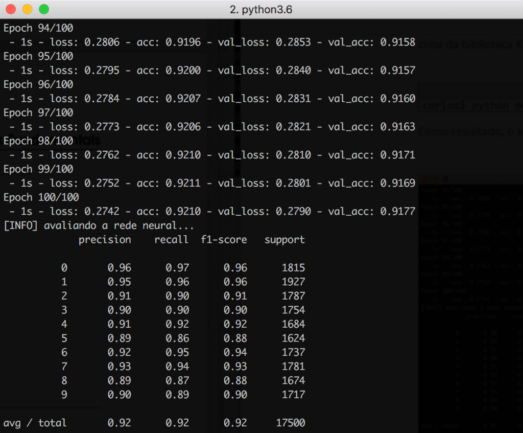
To evaluate the performance of the algorithm, we call the model.predict method to generate predictions on top of the test dataset. The model’s challenge is to make predictions for the 17,500 images that make up the test set, assigning a label from 0-9 to each one:

# evaluate the Neural Network
print("[INFO] evaluating the neural network...")
predictions = model.predict(testX, batch_size=128)
print(classification_report(testY.argmax(axis=1), predictions.argmax(axis=1)))

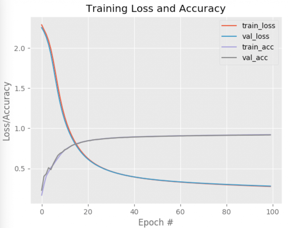
Finally, after obtaining the performance report, we will want to plot the accuracy and loss over the iterations. Visually analyzing allows us to easily identify situations of overfitting, for example:

# plot loss and accuracy for the 'train' and 'test' datasets
plt.style.use("ggplot")
plt.figure()
plt.plot(np.arange(0,100), H.history["loss"], label="train_loss")
plt.plot(np.arange(0,100), H.history["val_loss"], label="val_loss")
plt.plot(np.arange(0,100), H.history["acc"], label="train_acc")
plt.plot(np.arange(0,100), H.history["val_acc"], label="val_acc")
plt.title("Training Loss and Accuracy")
plt.xlabel("Epoch #")
plt.ylabel("Loss/Accuracy")
plt.legend()
plt.show()

Executing the Neural Network

With the code ready, you just need to execute the command below to see our Neural Network built on top of the Keras library in full operation:

$ python neural_network_keras.py

As a result, the classification_report shows that after 100 epochs, the network achieved an accuracy of 92%, which is a good result for this type of architecture. Just out of curiosity, Convolutional Neural Networks have the potential to reach up to 99% accuracy (!):

Obviously, there are many improvements that can be made to enhance the performance of our network, but even a simple architecture already delivers excellent performance.

Looking at the graph below, note how the curves related to the training and validation datasets are practically overlapping. This is a great indication that there were no overfitting problems during the training phase.

Summary

Well, reaching the end of the post, the basic concepts of Neural Networks were introduced, as well as the MNIST dataset, widely used to benchmark algorithms. By testing the performance of a neural network with 4 layers (input+2 hidden layers + output), we managed to achieve 92% accuracy in the predictions made.

The implementation was done using Keras, showing that with just a few lines of code, it is possible to build great classification models.

Finally, I would like to say that I intend to produce articles not only focused on code writing/implementation, but also delving deeper into the theoretical and mathematical concepts behind machine learning algorithms and methods.

I strongly believe that we only evolve when we get hands-on and go deeper into something. This is what I am doing for myself, and I hope to share these learnings here on the blog.