What if you could take a neural network that took weeks to train on millions of images and, in just a few minutes, adapt it to solve your specific problem? That is transfer learning, and it is probably the most important technique for anyone working with deep learning in practice.
Training a neural network from scratch requires a lot of data and computational power. But the truth is that most real-world problems don’t need that. The features a network learns when classifying roughly 1.28 million ImageNet images (edges, textures, shapes) are useful for almost any visual task. The idea behind transfer learning is simple: reuse that already acquired knowledge and adapt it to a new task.
In this article, we will apply transfer learning with PyTorch to classify 102 flower species using a ResNet18 pre-trained on ImageNet. We will compare two approaches: Feature Extraction (85.7% accuracy) and Fine-Tuning (92.5%), understand when to use each one and why the difference is so significant.
You can follow along with the complete notebook on Google Colab.
What Is Transfer Learning?
Imagine you are a French chef with 20 years of experience. If someone asks you to cook Japanese food, you don’t need to learn what salt, fire or a knife is. You already know how to cut, season, and control temperature. You just need to learn the specific techniques and ingredients of Japanese cuisine. All the foundational knowledge you accumulated is transferable.
With convolutional neural networks, it works the same way. A ResNet18 trained on ImageNet learned to detect edges in the early layers, textures in the intermediate ones and complex patterns in the deeper layers. These representations are generic enough to be useful in completely different tasks, such as classifying flowers, detecting industrial defects or identifying tumors in X-rays.
Transfer learning consists of taking a network pre-trained on a task with lots of data (such as ImageNet) and reusing it on a new task with less data. In practice, there are two main strategies:
- Feature Extraction: freeze all layers of the network and train only a new classifier on top.
- Fine-Tuning: unfreeze some layers and train them along with the classifier, allowing the network to adjust its representations for the new task.
The Dataset: Oxford Flowers 102
The Oxford Flowers 102 is a classic benchmarking dataset in computer vision. It contains images of 102 flower species found in the United Kingdom, with 1,020 training images, 1,020 for validation and 6,149 for testing. Each training batch contains 32 images (batch_size=32).
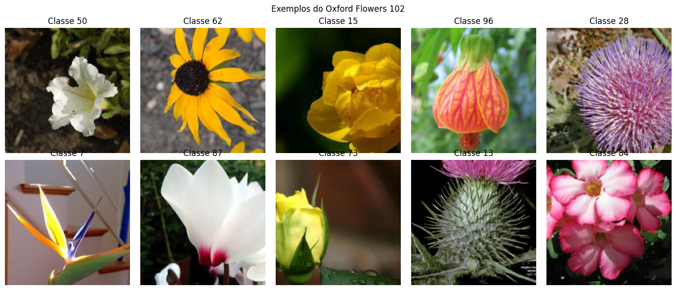
Notice the diversity: flowers of very different colors, shapes and sizes. Some species are visually similar, which makes classification challenging. With only 10 training images per class on average, training a network from scratch would be impractical. This is exactly the scenario where transfer learning shines.
train_transform = transforms.Compose([
    transforms.Resize(256),
    transforms.RandomCrop(224),
    transforms.RandomHorizontalFlip(),
    transforms.ToTensor(),
    transforms.Normalize([0.485, 0.456, 0.406],
                         [0.229, 0.224, 0.225])
])

test_transform = transforms.Compose([
    transforms.Resize(256),
    transforms.CenterCrop(224),
    transforms.ToTensor(),
    transforms.Normalize([0.485, 0.456, 0.406],
                         [0.229, 0.224, 0.225])
])

train_dataset = torchvision.datasets.Flowers102(
    root="./data", split="train", download=True, transform=train_transform
)
val_dataset = torchvision.datasets.Flowers102(
    root="./data", split="val", download=True, transform=test_transform
)
test_dataset = torchvision.datasets.Flowers102(
    root="./data", split="test", download=True, transform=test_transform
)

print("Training:", len(train_dataset), "images")
print("Validation:", len(val_dataset), "images")
print("Test:", len(test_dataset), "images")
# Training: 1020 | Validation: 1020 | Test: 6149
That is 1,020 training images for 102 classes. Too few for a neural network to learn from scratch, but enough to adapt a network that already knows how to “see”.
ResNet18 and the Domain Problem
Before applying transfer learning, it is worth understanding what the pre-trained ResNet18 already knows. It was trained on ImageNet, a dataset with 1,000 classes that include animals, vehicles, everyday objects. There are some generic flower classes (like daisy), but none of the 102 specific species from Oxford Flowers.
What happens when we show a flower to this network?
# Get a flower image directly from the dataset (fixed index for reproducibility)
img, label = train_dataset[0]

model_original = model_original.to(device)
img_gpu = img.unsqueeze(0).to(device)

with torch.no_grad():
    output = model_original(img_gpu)
    probs = torch.softmax(output, dim=1)
    top5_probs, top5_idx = probs.topk(5)

print("ResNet18 (ImageNet) predictions for a flower:")
for i in range(5):
    idx = top5_idx[0][i].item()
    prob = top5_probs[0][i].item()
    print(f"  {imagenet_labels[idx]:>30s}: {prob:.1%}")
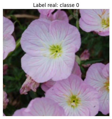
The network recognizes it is a flower: daisy appears with 69.2% confidence, followed by pot (6.4%), bee (5.1%), vase (5.0%) and small white (2.3%). It gets the generic category right, but cannot distinguish between the 102 species from Oxford Flowers because it was never trained at that level of granularity. The internal features are good (it understands shapes, colors, textures), but the final classification layer maps to the 1,000 ImageNet classes, not to our 102.
This is exactly what we will fix with transfer learning: keep the features and replace the classifier.
Feature Extraction: Freezing the Network
The first approach is the simplest. We take ResNet18, freeze all weights (no convolutional layer is updated during training) and replace only the last fully connected layer with a new one, with 102 outputs (one for each flower species).
model_fe = resnet18(weights=ResNet18_Weights.IMAGENET1K_V1)

# Freeze all backbone parameters
for param in model_fe.parameters():
    param.requires_grad = False

# Replace the fc layer for 102 classes
# (new modules are created with requires_grad=True by default)
num_features = model_fe.fc.in_features
model_fe.fc = nn.Linear(num_features, 102)

total = sum(p.numel() for p in model_fe.parameters())
trainable = sum(p.numel() for p in model_fe.parameters() if p.requires_grad)
print(f"Total: {total:,} | Trainable: {trainable:,} ({100*trainable/total:.1f}%)")
# Total: 11,228,838 | Trainable: 52,326 (0.5%)
Out of 11.2 million parameters, we are training only 52,326 (the weights of the new fc layer: 512 x 102 + 102 bias). The convolutional network works as a fixed feature extractor, and the classifier on top learns to map those features to the 102 species.
After 15 epochs of training, the results:
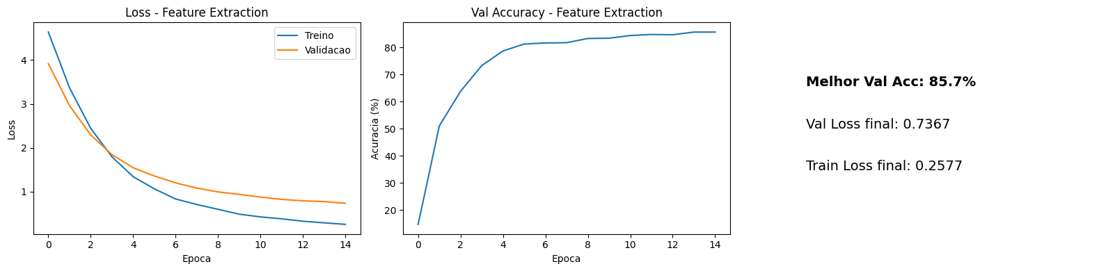
Validation accuracy reached 85.7% with a final val loss of 0.7367. That is an impressive result for 102 classes with so little training data and only the final layer being trained. On the test set (6,149 images), the model achieved 83.7% accuracy. The convolutional network, even frozen, already extracted features discriminative enough to separate most species.
But 85.7% is not the ceiling. The generic ImageNet features are good, but not perfect for flowers. Can letting the network adjust its representations improve the result?
Fine-Tuning: Unfreezing Part of the Network
In fine-tuning, we unfreeze some of the convolutional layers and allow them to adapt to the new domain. The intuition is that the early layers (which detect edges and basic textures) are universal, but the deeper layers (which detect complex patterns) can benefit from adjustment to the flower domain.
The most common strategy is to unfreeze the last layers of the network. In ResNet18, we unfreeze layer4 (the last residual block) and the new fc layer.
model_ft = resnet18(weights=ResNet18_Weights.IMAGENET1K_V1)

# Freeze everything first
for param in model_ft.parameters():
    param.requires_grad = False

# Unfreeze layer4
for param in model_ft.layer4.parameters():
    param.requires_grad = True

# Replace fc (new modules are created with requires_grad=True)
model_ft.fc = nn.Linear(model_ft.fc.in_features, 102)

total_params = sum(p.numel() for p in model_ft.parameters())
trainable_params = sum(p.numel() for p in model_ft.parameters() if p.requires_grad)
print(f"Trainable: {trainable_params:,} / {total_params:,} ({100*trainable_params/total_params:.1f}%)")
# Trainable: 8,446,054 / 11,228,838 (75.2%)
Now we are training 8.4 million parameters (75.2% of the total). An important detail is using different learning rates for each part of the network. The fc layer is new and needs to learn from scratch, so it uses a higher learning rate. layer4 already has good weights and only needs fine adjustments, so it uses a lower learning rate.
# Differential learning rates
optimizer_ft = optim.Adam([
    {"params": model_ft.layer4.parameters(), "lr": 1e-4},   # fine adjustment
    {"params": model_ft.fc.parameters(), "lr": 1e-3},       # new layer
])
This technique is called differential learning rate (or discriminative learning rates). The idea is that deeper layers, which already have reasonable representations, should be updated with smaller steps to avoid destroying the pre-trained knowledge. Here, layer4 trains with a learning rate 10 times smaller than the fc layer.
After 15 epochs of training:
- Validation accuracy: 92.5%
- Test accuracy: 90.2%
- Final val loss: 0.3378
The improvement is significant. Validation accuracy went from 85.7% to 92.5%, and val loss dropped from 0.7367 to 0.3378. On the test set (6,149 never-before-seen images), the model correctly classified 90.2% of them.
Feature Extraction vs Fine-Tuning
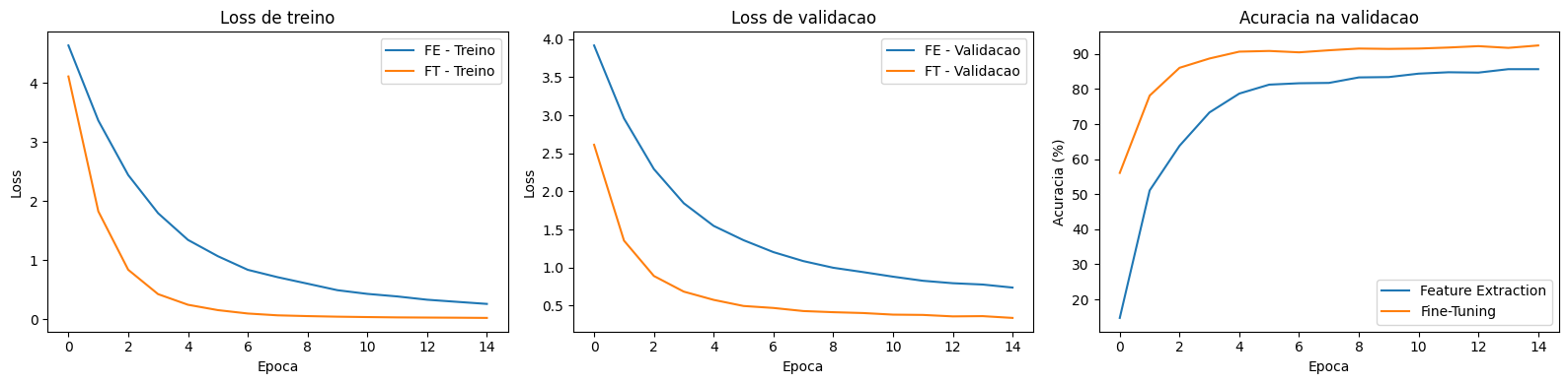
The visual comparison makes clear what the numbers already indicated. Fine-tuning converges to a much lower loss and a consistently higher accuracy. Let’s organize the results:
| Metric | Feature Extraction | Fine-Tuning |
|---|---|---|
| Trainable parameters | 52,326 (0.5%) | 8,446,054 (75.2%) |
| Validation accuracy | 85.7% | 92.5% |
| Test accuracy | 83.7% | 90.2% |
| Final val loss | 0.7367 | 0.3378 |
| Learning rate | 1e-3 (fc) | 1e-4 (layer4), 1e-3 (fc) |
Feature extraction is faster to train (fewer parameters, no backpropagation through the convolutional layers) and more resistant to overfitting. It is the best choice when you have very little data or need a quick result.
Fine-tuning delivers superior results when you have enough data to adjust the convolutional layers without overfitting. The differential learning rate is essential here: without it, a high learning rate can destroy the pre-trained representations (so-called catastrophic forgetting), and a learning rate too low would make training the fc layer slow.
When to Use Each Approach?
The choice between feature extraction and fine-tuning depends on two factors: the amount of data and the similarity between the original and the new domain.
If the new dataset is small and similar to ImageNet (animals, common objects), feature extraction is usually sufficient. If it is large or very different (medical images, satellite, microscopy), fine-tuning is almost always the better option.
When in doubt, start with feature extraction as a baseline. If the result is not satisfactory, move to fine-tuning by unfreezing the last layers. This is a progressive approach that minimizes the risk of overfitting. To understand what the network learned to look at after fine-tuning, see how to use Grad-CAM to visualize where the CNN focuses when classifying each flower.
Takeaways
- Transfer learning reuses knowledge: instead of training from scratch, we use a network pre-trained on ImageNet as a starting point. The generic features (edges, textures, shapes) are transferable to almost any visual task.
- Feature extraction is simple and effective: by freezing the network and training only the final layer, we reached 85.7% validation accuracy and 83.7% on the test set across 102 flower classes with just 52 thousand trainable parameters.
- Fine-tuning delivers superior results: by unfreezing
layer4of ResNet18 and using differential learning rate (1e-4 for pre-trained layers, 1e-3 for the new layer), accuracy rose to 92.5% on validation and 90.2% on the test set.
- Differential learning rate prevents catastrophic forgetting: pre-trained layers should be updated with smaller steps to preserve acquired knowledge, while new layers need larger steps to learn quickly.
- Start simple, evolve if needed: feature extraction as a baseline, fine-tuning when you need more accuracy. This progressive approach is the safest path in practice.