Vision Transformer (ViT): Python Implementation

What if I told you that a model originally created to translate text can analyze images with performance comparable to — and in some cases better than — Convolutional Neural Networks?

That’s exactly what the Vision Transformer (ViT) proposes. And the idea behind it is so elegant it fits in a single sentence: Cut the image into pieces, treat each piece as a “word,” and let the Transformer do the rest.

The Vision Transformer (ViT) was introduced by Dosovitskiy et al. in the paper An Image is Worth 16×16 Words, published in 2020, and quickly established itself as one of the most influential architectures in modern computer vision.

In this article, I’ll walk you through every component of the ViT architecture, from patch creation to the final classification step. At the end, we’ll put it all into practice using a pre-trained model to classify a real image and visualize the attention maps, understanding how the model distributes its focus across the image.

💡 Notebook: Vision Transformer ViT

 

What Is the Vision Transformer?

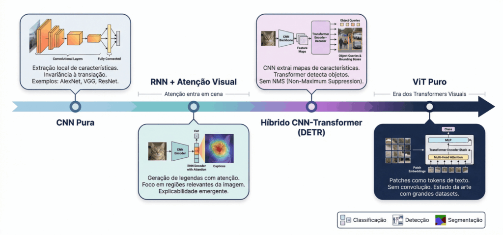
Until 2020, the world of computer vision was dominated by Convolutional Neural Networks (CNNs). From LeNet-5 in the 90s to ResNet in 2015, the paradigm was always the same: local filters sliding across the image, extracting hierarchical patterns.

The problem with CNNs is that they see locally. Each filter looks at only a small region of the image at a time. For distant information to communicate, you need to stack many layers.

ViT proposed something radical: throw away convolutions entirely and use only Transformers. The same architecture that revolutionized natural language processing (GPT, BERT) was applied directly to images.

The result? When trained with enough data, ViT outperformed the best CNNs of the time.

Patches: Cutting the Image into Pieces

The first question is: how do you feed an image into a Transformer? The Transformer works with sequences of tokens (like words in a sentence). An image is a grid of pixels, not a sequence.

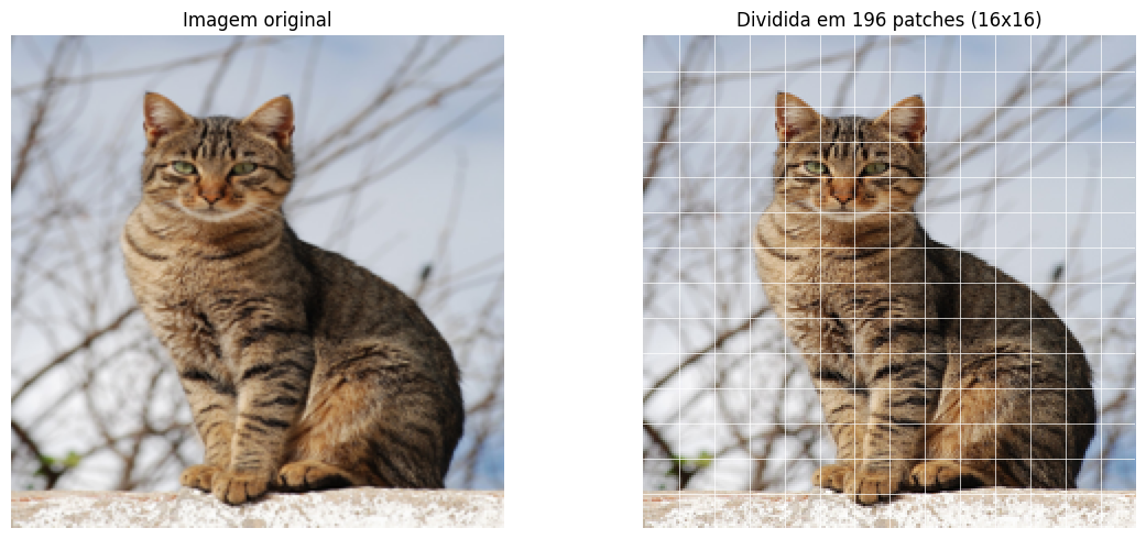
ViT’s solution is simple and ingenious: divide the image into a grid of squares called patches. Each patch is a piece of the image, like a puzzle piece.

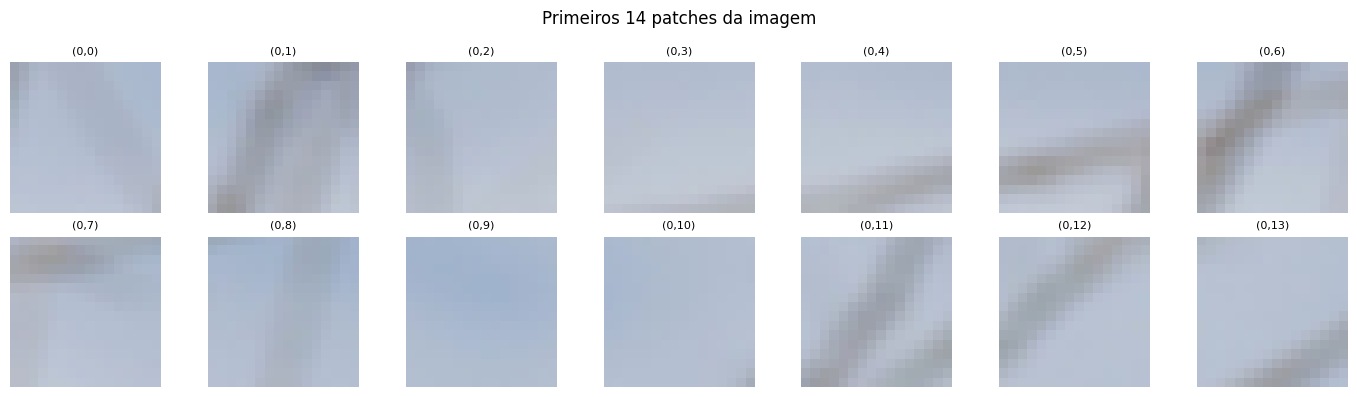
A 224×224 pixel image divided into 16×16 patches produces a 14×14 grid, that is, 196 patches. Each patch captures a local region of the image: an eye, a piece of the background, part of a paw.

Think of it this way: if a text Transformer processes a sequence of words, ViT processes a sequence of patches. Each patch is a “visual token.”

# Split a 224x224 image into 16x16 patches
patch_size = 16
img_size = 224
n_patches_side = img_size // patch_size
n_patches_total = n_patches_side ** 2

print(f"Grid: {n_patches_side}x{n_patches_side} = {n_patches_total} patches")
# Grid: 14x14 = 196 patches

Looking at the patches individually, we can see that each one captures a different region of the photo: some contain parts of the cat, others pieces of the background or branches.

Patch Embedding: From Pixels to Vectors

Each patch is a pixel matrix (16×16×3 for RGB images). But the Transformer works with fixed-dimension vectors. We need to convert each patch into a numerical vector (this is the patch embedding).

In practice, ViT uses a convolution with kernel and stride equal to the patch size. This operation does two things at once: it divides the image into patches and projects each patch into a vector of dimension D.

# Conv2d with kernel=16 and stride=16: splits and projects in one operation
embed_dim = 768  # ViT-Base dimension
patch_embed = nn.Conv2d(3, embed_dim, kernel_size=16, stride=16)

# Input: (1, 3, 224, 224)
# After convolution: (1, 768, 14, 14)
# Reshaped: (1, 196, 768)

The result is a sequence of 196 vectors, each with 768 dimensions. Each 16×16×3 pixel patch (768 values) became a 768-dimensional vector — a compact numerical representation of that image region.

CLS Token and Positional Embedding

Before entering the Transformer, two ingredients are added to the sequence.

The CLS token (from classification) is a special vector inserted at the beginning of the sequence. It acts as an “observer” that doesn’t belong to any specific patch. As it passes through all the attention layers, the CLS token accumulates information from every patch. In the end, it’s the one we use to classify the image.

The Positional Embedding solves a fundamental problem: the Transformer has no notion of order. Without it, the model wouldn’t know that the patch in the top-left corner is different from the one in the bottom-right corner. We add a position vector to each token, giving the model the information of “where” each patch was in the original image.

The resulting sequence has 197 tokens (1 CLS + 196 patches), each with 768 dimensions. This is the Transformer’s input.

Self-Attention: The Central Piece

The self-attention mechanism is what makes the Transformer so powerful. It allows each token to “look at” every other token and decide who to pay attention to.

The most useful analogy is that of a classroom. Imagine each patch is a student. Each student generates three things:

• Query (Q): “What am I looking for?”
• Key (K): “What do I have to offer?”
• Value (V): “What information do I carry?”

Attention is calculated by comparing each token’s Query with the Keys of all other tokens. The more compatible Q and K are, the more attention one token pays to the other. The result is a weighted average of the Values.

   

The division by prevents values from becoming too large before the softmax. It’s a simple detail, but crucial for training stability.

In practice, ViT doesn’t use a single attention — it uses Multi-Head Attention. The idea is to split the embedding into multiple “heads” that operate in parallel, each learning to attend to different aspects: one head might focus on colors, another on shapes, another on textures. The outputs are concatenated at the end.

The Transformer Block

Each Transformer block combines two operations, both with residual connections and Layer Normalization:

1. Multi-Head Self-Attention — tokens communicate with each other
2. Feed-Forward Network (FFN) — each token is individually processed by two linear layers with GELU activation

The structure is:

tokens → LayerNorm → Multi-Head Attention → (+residual) → LayerNorm → FFN → (+residual)

ViT-Base stacks 12 of these blocks in sequence. With each layer, the tokens become richer in contextual information. The CLS token, which started with no information, progressively “listens” to all patches and builds a global representation of the image.

The residual connections (adding the input to the output) facilitate gradient flow during training and allow the model to stack many layers without degrading the signal.

In Practice: Classifying a Cat Photo

The truth is, in day-to-day work, nobody implements ViT from scratch. We use pre-trained models and run inference or fine-tuning. torchvision already includes ViT-B/16 pre-trained on ImageNet with 1,000 classes.

Let’s load the model and classify a real cat photo:

from torchvision.models import vit_b_16, ViT_B_16_Weights

# Load pre-trained model on ImageNet
weights = ViT_B_16_Weights.IMAGENET1K_V1
model = vit_b_16(weights=weights)
model.eval()

# Preprocess and classify
preprocess = weights.transforms()
img_input = preprocess(img).unsqueeze(0)

with torch.no_grad():
    output = model(img_input)
    probabilities = F.softmax(output[0], dim=0)

# Top-5 predictions
top5_prob, top5_idx = torch.topk(probabilities, 5)
categories = weights.meta["categories"]

for i in range(5):
    print(f"  {categories[top5_idx[i]]:30s} {top5_prob[i].item():.1%}")

The result:

  tiger cat                      66.2%
  tabby                          16.1%
  Egyptian cat                    8.3%
  lynx                            0.2%
  tiger                           0.1%

The model classified the image as tiger cat with 66.2% confidence, followed by tabby (16.1%) and Egyptian cat (8.3%). The top three classes are all domestic cat categories — the model nailed it. All of this without any training, using only pre-trained ImageNet weights.

Visualizing Attention: Where Is the ViT Looking?

One of the great advantages of the Vision Transformer is its interpretability. We can visualize which regions of the image were most important for the model’s decision.

To do this, we use a technique called attention rollout. Instead of looking at the attention of a single layer (which tends to be sparse and hard to interpret), rollout accumulates the attention weights from all 12 layers, taking residual connections into account.

The result is a map that shows, in aggregate, where the CLS token concentrated its attention throughout the entire network.

# Collect attention from each block and accumulate via rollout
rollout = torch.eye(197).unsqueeze(0)  # identity matrix
for attn in all_attn:
    attn_with_residual = attn + torch.eye(197).unsqueeze(0)
    attn_with_residual = attn_with_residual / attn_with_residual.sum(dim=-1, keepdim=True)
    rollout = attn_with_residual @ rollout

# Extract attention from CLS to the 196 patches
cls_attn = rollout[0, 0, 1:].reshape(14, 14).numpy()

The brighter regions in the map indicate where the model concentrated more attention to classify the image. Notice how the attention focuses on the cat’s body and head, ignoring the background with branches and the sky. The ViT learned, without explicit supervision, to focus on the most discriminative regions of the image — exactly what a human would do.

ViT vs CNN: When to Use Each?

CNNs process images with local filters and build spatial hierarchies layer by layer. They are efficient and work well even with limited data. ViT, on the other hand, processes the image globally from the very first layer.

In other words, each patch can relate to any other patch, regardless of distance.

This global capability comes at a cost: ViT needs much more data to learn good representations from scratch. In the original paper, ViT only outperformed CNNs when pre-trained on massive datasets like JFT-300M (300 million images). For smaller datasets, CNNs still hold the advantage.

In practice, the most common strategy is to use transfer learning: start from a ViT pre-trained on a large dataset and fine-tune it for your specific task.

Key Takeaways

• Image as a sequence of patches: ViT splits the image into 16×16 pieces and treats each one as a “token,” applying the same Transformer architecture used in NLP — with no convolutions whatsoever.

• Patch embedding via convolution: a Conv2d with kernel and stride equal to the patch size splits the image and projects each patch into a 768-dimensional vector in a single operation.

• CLS token as a global observer: a special token inserted at the beginning of the sequence accumulates information from all patches via attention, serving as the image’s global representation for classification.

• Self-attention enables global communication: unlike CNNs that see locally, each patch in ViT can directly relate to any other patch in the image, capturing long-range dependencies from the very first layer.

• In practice, use pre-trained models: torchvision’s ViT-B/16 classified our cat photo as tiger cat with 66% confidence, and the attention map confirmed the model focuses on the animal while ignoring the background — all with direct inference, no additional training required.